rtklibexplorer

Configuring the Quectel LC29HEA receiver for real-time RTK solutions

This is a follow up to my previous post in which I describe my first experience with the Quectel LC29H receiver. In this post I will go over the details on how I configured the rover and base receivers for a real-time RTK solution. These instructions are specifically for the LC29HEA receiver boards I bought on AliExpress, but, except for the references to the UART/USB slide switches, should work on any receiver board with an LC29HEA module.

The commands to configure the receiver are all described in the LC29H Protocol Specification, although it is not completely up to date with the latest firmware. Specifically, I had to read the latest firmware notes to find that 2 Hz and 5 Hz are now options for the position output rate. The commands all consist of strings of ASCII characters, but require a checksum at the end of the command. The easiest way to send and receive these commands is by using the command console window in the Windows QGNSS app from Quectel since it will generate the checksums for you with the click of a button.

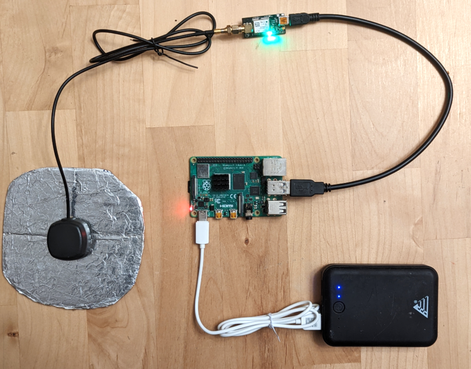
To get started, download the app, open it up, connect the receiver to your computer with a USB cable, and connect an antenna to the receiver with the SMA connector. Check that the two slide switches on the receiver board are both set down towards the “USB” label.

Then use the “Set Device Information” option in the Device tab (or the “gear” icon in the toolbar) to find and configure the receiver communication settings. Set the Model to “LC29HEA” and the baudrate to 460800 as shown below.

Once this is done, open up a “Text Data” window from the “View” menu and you should see a string of NMEA text messages scrolling through the window assuming your receiver is in its default configuration. It should look something like this:

Next, open up a “Command console” window from the “Tools” menu which we will use to send configuration commands to the receiver.

Rover Configuration:

The next step is to enter the commands into the command console. We will first set up the rover. I’ve listed the command I used to do this below so that they can be cut and pasted into the QGNSS console. Note that the comments are for information only and should not be copied. I’ve also included the checksum for each command which can be copied or generated by using the “Checksum” button. Be aware that some commands don’t take effect until the parameters are saved to flash or the module is rebooted.

$PQTMRESTOREPAR*13 # restore PQTM params to default and reset
$PQTMCFGRCVRMODE,W,1*2A # set receiver to rover mode
$PQTMSAVEPAR*5A # save PQTM params to flash
# manually power cycle module
$PAIR062,2,0*3C # turn off GSA messages
$PAIR062,3,0*3D # turn off GSV messages
$PAIR062,5,0*3B # turn off VTG messages
$PQTMCFGNMEADP,W,3,6,3,2,3,2*37 # set decimal precision for NMEA
$PAIR050,200*21 # set pos output interval to 200 ms
$PQTMSAVEPAR*5A # save PQTM params to flash
# manually power cycle module

QGNSS Command Console Window ( commands to configure rover)

Once you’ve entered all the commands into the console, you can run them by consecutively pressing the “Send” button for each command. If you have made any modifications to any of the commands you will need to press the “Checksum” button first to recalculate all of the checksums.

These instructions assume the firmware on the module is no older than LC29HEANR11A03S_RSA which has an associated date of 10/31/23. You can use the command at the end of the screenshot above to check the version of firmware on your module. If your firmware is older than this, then I believe the only change you will need to make to these instructions is that the 5 Hz option is not supported and you will need to set the PAIR050 option to 100 instead of 200 which will set the output rate to 10 Hz instead of 5 Hz.

Base Configuration:

If you are going to use a second LC29H for a local base receiver, you will need to go through a similar process to configure that module. These are the commands I used:

$PQTMRESTOREPAR*13 # restore PQTM params to default and reset
$PQTMCFGRCVRMODE,W,2*29 # set receiver to base mode
$PQTMSAVEPAR*5A # save PQTM params to flash
# manually power cycle module
$PAIR432,1*22 # output RTCM3 MSM7 messages
$PAIR434,1*24 # output RTCM3 antenna position (1005)
$PAIR062,0,01*0F # Enable NMEA GGA message
$PQTMCFGSVIN,W,2,0,0,x,y,z*3B # set base location in XYZ coords
$PQTMSAVEPAR*5A # save PQTM params to flash
# manually power cycle module

Note that for the PQTMCFGSVIN command, you will need to use the XYZ coordinates of your base station and update the checksum before sending. Alternatively, the LC29H supports a survey-in capability to automatically generate an approximate base position.

Once you have sent this sequence of commands to the receiver, open up a “Binary data” window from the “View” menu and you should see the RTCM3 MSM observation messages and the 1005 base location message.

RTCM3 messages in QGNSS Binary data window

One minor issue I found is that the PAIR432 command to enable RTCM3 MSM7 messages does not seem to get saved to flash properly, so after cycling power, the module will switch to outputting MSM4 messages rather than MSM7. These contain slightly less information than the MSM7 messages but in most cases this should have negligible to no effect on the RTK solution. The MSM4 messages also require less bandwidth.

RTK Solution:

Once you are getting the correct outputs from both receivers, or a single receiver and external base correction stream, it is time to link them together to get an RTK solution. If you are using an LC29H as a local base station, you will want to connect it to an NTRIP caster to broadcast the correction stream. I describe one way of doing this with RTK2GO in this post. Once this is up and running, or you have access to NTRIP corrections from an external L1/L5 base station, the next step is to feed the base corrections to the rover using an NTRIP client. In my experiment I used an RTKLIB STRSVR stream server to do this, but for just checking out the receiver, it is simpler to use the NTRIP client tool built into QGNSS. Open this window from the “Tools” menu in QGNSS and configure it with your NTRIP address, username, password, port, and mountpoint. Once it is configured, set the “Connect to Host” button to on. If you are in an open sky view and have a ground plane under your antenna, you should see the “Quality indicator” field in the QGNSS output window switch to “Float RTK” and then to “Fixed RTK” as seen in the screenshot below. In this case, you can see from the RTK Float count field that it took 41 samples to converge from float to fix. Since the output rate is set to 5 Hz, this is about 8 seconds. The time to fix will vary depending on sky view, atmospheric conditions, and antenna quality.

So, that’s it, you should be up and running now and ready to collect some position data with centimeter-level accuracy. If you find any issues with these instructions or improvements to them, please leave a comment below.

Dual frequency RTK for less than $60 with the Quectel LC29HEA

The u-blox F9P dual-frequency RTK receiver has been my go-to choice for high precision RTK or PPK solutions ever since it first came out in 2018. Available initially on a receiver board with antenna for under $300, it offered a performance and price point far better than anything that preceded it. However, that was six years ago and although the price for the F9P receiver and antenna has come down a little to around $250 since then and they now offer a few more variations, it feels like u-blox hasn’t introduced anything dramatically new in a fairly long time.

Meanwhile, there have been a number of lower cost dual-frequency receivers introduced recently from other companies which look quite promising. I hope to take a look at a few of these eventually, but have decided to start with the LC29H from Quectel.

The F9P is an L1/L2 receiver, while the LC29H, like most of the newer receivers is an L1/L5 receiver. The L5 signals have some advantages over the L2 signals, but (like the L2C signals used by the F9P and other low-cost L1/L2 receivers) are not yet available on all satellites.

The LC29H module comes in several variants. The newest ones most generally available on receiver boards are the DA, BS, and EA variants. The specs for these are shown below. The EA variant is the one most recently available and is the only one that will output raw observations or RTK solution points at greater than 1 Hz. A 1 Hz sample rate is fine for static applications, but for dynamic rovers a higher sample rate is usually necessary. For this reason, I will focus on the LC29HEA.

Quectel LC29H specs for DA, EA, and BS variants

Probably because it’s relatively new, it is a little more difficult to find receiver boards built with the EA module. I ended up ordering two receivers from this link on AliExpress. If the link no longer works by the time you read this post, you can probably find something similar using their search option. The price for this one was $57.69 for the receiver and antenna plus $4.79 shipping to the U.S. In my case, the boards arrived in less than two weeks with no issues. I ordered the boards without the antennas since I missed the combined option when I made the order. For my initial evaluation I used what I’m guessing is a similar low-cost L1/L5 antenna from Waveshare for $17. Waveshare also sells LC29H receivers but at the current time, only with the AA, BS, and DA variants.

Quectel LC29HEA receiver with L1/L5 antenna from AliExpress

To start with, I chose to compare a real-time internal RTK solution using a pair of F9P receivers for base and rover to a real-time internal RTK solution using a pair of LC29HEA receivers. If I was trying to compare the two receivers directly, I would use the same antenna for both rovers. However, for this experiment, I wanted to compare a lower cost solution that included both a lower cost receiver and a lower cost antenna. This means that the results can not be used to draw any conclusions regarding differences between the receivers directly, only differences between the combinations of receiver and antenna. I hope to do another comparison later using a single antenna to more directly compare the receivers.

I connected the two base receivers through an antenna splitter to a Harxon geodetic GPS-500 antenna on my roof. Although this antenna is advertised as L1/L2 only, I have found it gives signal strengths in the L5 band equivalent to L1/L2 so felt it was fair to use in this comparison. I connected the F9P rover to a u-blox ANN-MB L1/L2 antenna and the LC29H rover to the low-cost L1/L5 antenna from Waveshare.

I have done most of my previous comparison tests with antennas on top of vehicles. For this test I chose something a little more challenging, and walked around my backyard, sometimes in the relative open, sometimes close to large trees, and sometimes close to the house, but never underneath dense tree foilage.

I configured the base receivers to output RTCM3 MSM7 observation messages at 1 Hz and broadcast them to the internet using the RTKLIB STRSVR stream server app and a couple of RTK2go NTRIP servers similar to what I describe in this post.

The LC29H can only be configured to output RTK positions at 1 Hz or 10 Hz, so I chose 10 Hz for the LC29H rover. [Note 5/1/24: the release notes for the latest firmware indicate that options for 2 Hz and 5 Hz have just been added] According to the datasheet, the F9P has a maximum RTK position output of 7 Hz when running with all four GNSS constellations but for this experiment I left it at 5 Hz which I find an adequate sample rate for most applications.

Using a laptop running four instances of STRSVR, I configured two of these to stream the NTRIP corrections coming from the two base receivers to go to the two rover receivers over USB cables. I used the other two to stream the real-time output of the two rovers to a couple of files. I describe a similar setup for just the F9P in this post. I used the u-blox u-center app to configure the F9P, and the Quectel QGNSS app to configure the LC29H. The LC29H configuration commands are somewhat cryptic and need to be typed into a command console in the Quectel app, so this was not as easy as configuring the F9P, but the details for doing this are reasonably well documented in the Quectel LC29H Protocol Spec.

I will share the details of exactly how I configured the LC29H base and rover modules in a separate post. The biggest issue I found here was that when running at 10 Hz, not all features can be enabled at the same time and the way the module handles this can sometimes be confusing. For example, you can not output RTCM observation messages and 10 Hz RTK real-time positions at the same time. This setup is not necessary for this experiment but can be useful if you want real-time position information but also want to postprocess the raw observations later with RTKLIB. Also, some commands would take effect immediately and others only after config parameters were saved to flash, or when the module was reset.

After all four receivers were configured, I walked around the backyard with the laptop connected to the two rovers, and the two rover antennas mounted together about 30 cm apart. When close to the house or the trees I was careful to keep the spacing between both antennas and the obstruction similar to each other.

RTKPLOT will plot two real-time NMEA position streams, so I also had an instance of this running on my laptop to plot the two solutions real-time. The screenshot below is from my laptop while I was running the experiment, showing the four stream server windows and the RTKPLOT window. The yellow/green plot lines are float/fix status for the F9P and the olive/blue plot lines are float/fix status for the LC29H. I took this screenshot before I started walking around. The antennas were static and I was periodically covering both antennas to force loss-of-lock and reconvergence of the two solutions. Both receivers recovered a fix status in a reasonable time but the F9P was generally two to three times faster.

Screenshot of my laptop while collecting data

The screenshot below shows the real-time RTK position output for the F9P collected while walking around. As you can see, most of the solution is fixed, but close to the house and close to the tree line on the right where the trees are tallest and thickest, there is more float solution. The points closest to the house are actually under the eaves of the roof. The float points in the lower middle of the image are from when I was covering and uncovering the antenna as I described above. I generated this image using the POS2KML app in RTKLIB to generate a KML file and then displayed it with Google Earth.

Here is the same image for the LC29H real-time RTK solution. Again, most of the open-sky area is fixed but a higher percent of the more challenging regions are float.

I don’t have a ground truth for this data so I can’t directly compare the accuracy of the two solutions. What I can do is plot the difference between the two solutions to get a general idea of the solution errors. Since the antennas are a fixed distance apart, the difference between the two solutions should be a circle with radius equal to the antenna separation distance, assuming the antennas were kept fairly close to level while the data was taken. Here’s the result of plotting the solution difference with RTKPLOT

A large percentage of the points are on the circle, in this case with radius 34 cm, but there are also a fair number of points not on the circle. Given the challenging nature of this experiment, this is somewhat expected. Float points (yellow) off of the circle are less concerning since we know the accuracy is lower for them. Fix points (green) off the circle however are more concerning and generally indicate false fixes. Plotting both solutions versus time and comparing the vertical components can help tell us where the false fixes are and which solution they occurred in. This is because the trajectory covers the same ground multiple times so we know what the valid range of altitude is. The region below circled in red indicates both solutions are fixed but differ by well over the expected accuracy of a fixed solution. Since the blue (LC29H) solution is outside the range of altitudes from the rest of the data we can determine that this is the incorrect solution in this case.

F9P solution (green/yellow) and LC29H solution (olive/blue)

Based on the results of this single experiment, it appears that the Quectel LC29H with a very low cost antenna performed reasonably well in challenging conditions and deserves further investigation. It did not perform as well as the u-blox F9P with a more expensive antenna in these conditions, however given that it cost roughly one quarter as much, I think it did quite well. In less challenging conditions such as onboard a drone where sky views are generally less obstructed, I would expect the differences to be smaller.

Performance and cost are important, but of course they are not the only factors to consider when selecting a receiver. I did find that overall the documentation is more complete for the F9P, it is both easier to configure and more configurable than the LC29H, and there are some features such as event logging that are available on the F9P but not the LC29H.

One last thing to consider is that the overall performance results are a combination of, among other things, the antenna, the front end of the receiver and the internal RTK solution. I hope to do further experiments using a common L1/L2/L5 antenna and post-processing with RTKLIB to measure the differences in each of these components separately.

Well, I think that is enough for now. I hope to follow up with some more posts as I gain a little more experience with this receiver and eventually take a look at some other very low cost L1/L5 receivers as well.

If you have worked with the LC29H and would like to share your thoughts and experiences, please leave a comment below.

2023 Google Smartphone Decimeter Challenge

Google has just kicked off the 2023 Smartphone Decimeter Challenge on Kaggle. Similar to the previous two years, it is a competition to see who can generate the most accurate solutions for a large number of raw observation data sets collected with Android phones on vehicles driven around the Bay Area and Los Angeles. In the previous two competitions, all the phones were higher-end models that supported dual-frequency GNSS. This year, they are also including mid-range phones with only single frequency GNSS to better represent the total population of phones. This will make the solutions more challenging.

They have also increased the total prize money from $10,000 to $15,000. The competition started just over a week ago and will run until May 23 next year. The top three winners will be invited to present papers on their solutions at the 2024 ION GNSS+ conference.

Last year, after the competition had concluded, I shared a version of my final solution in a notebook on the competition’s Kaggle page. When copied to a local computer and run, it will generate a result that can be submitted to Kaggle and will place 5th in last year’s public leaderboard.

I have just published an updated version of this notebook on this year’s Kaggle page. It is the same solution as the previous version, just updated to run with this year’s data and also modified so it will run more easily on Linux as well as Windows. For anyone interested in joining the competition, this latest version will produce a score of 1.80 meters, which at the moment is good enough for first place. I’m sharing it to help promote a stronger competition as well as to encourage the use of RTKLIB.

Below is a screenshot of the state of the public leaderboard as of September 21. You can see the most recent version of the leaderboard here.

For reference, last year’s winning score on the public leaderboard was 1.38 meters, and I expect this year’s winning score to be lower. So, this is only a starting point, but it should give anyone interested in competing an opportunity to take advantage of previous work and jump in near the front of the pack (at least for the moment).

I’m happy to answer any questions about using RTKLIB in the competition but the rules require that I do that in the competition’s Kaggle discussion group so that the information is available to all participants. There was quite a bit of collaboration between competitors in last year’s competition as well as a lot of information shared after the competition, all on the competition’s Kaggle discussion group page, so check that out if you haven’t already.

More details of the optimizations I have made to RTKLIB for smart phone observations are described in these links:

Kalman Filter Adjustments in RTKLIB (the Options-Statistics tab)

In this post, I am going to describe how the Kalman filter in RTKLIB is configured and how it can be adjusted. In most cases, the default values work fine and there is no need to adjust these parameters, but in some cases it can be useful. Also, understanding these parameters can provide useful insight into how RTKLIB generates its solutions.

If you are interested primarily in how to set these values and not in what they do, then you may want to jump down to the end of the post where I discuss a few examples of where I have found adjusting these values to be helpful.

Parameters to enable and disable various filter states are sprinkled over the different tabs in the options menus of RTKPOST and RTKNAVI but the parameters that determine the inner details of the Kalman filter calculations are all listed on the Statistics tab as shown below.

Note that the parameters are divided into two sections, measurement errors and process noises. In a Kalman filter, each measurement will have a measurement error estimate associated with it, and each filter state will have a process noise estimate associated with it, both defined in terms of standard deviations (or sigmas). The Kalman treats all of the measurement errors as normally distributed with zero mean. In general, increasing the error estimates of the measurements relative to the process noises will cause the filter to rely more on the model, and reducing the error estimates of the measurements will cause the filter to rely less on the model and more directly on the measurements.

The description below will apply specifically to differential solutions (RTK/PPK) but the PPP solutions use a similar method.

MEASUREMENT ERRORS:
The primary measurement inputs to the Kalman filter are code and phase observations. The amount of error in each observation will be determined by many factors which we cannot determine directly, but in general, both satellite elevation and signal strength will correlate with measurement error. Since the receiver reports a signal strength (C/N0) for each measurement and we can determine the satellite elevation from the ephemeris messages, we can use either or both of these to generate an estimate of the error. For differential solutions (RTK/PPK), errors will also increase as the baseline between rover and base increases. Another option that is sometimes available is to use an error estimate provided directly by the receiver.

The original (2.4.3) version of RTKLIB uses the sum of four squared terms to determine the error estimate as a variance for each phase observation. The first term is a constant, the second term is a constant divided by the sine of the satellite elevation, the third term is a constant multiplied by the distance between base and rover, and the fourth term is a constant multiplied by the time since the last observation. The default values for the first two constants are three mm, and the third is zero. The last term is included to account for satellite clock stability and defaults to 5e-12 sec/sec. These are listed in the options tab as “Carrier-Phase: a+b/sinEl”, “Carrier-Phase: Baseline”, and “Satellite Clock Stability”.

The demo5 version of RTKLIB defaults to the same algorithm and values as the 2.4.3 code but has three additional terms which all default to zero. The first two terms allow the error estimate to be adjusted by the signal strengths of the base and rover observations using the formula a*10^(.1*MAX(snr_max – snr), 0). The two additional terms are a and snr_max in the above equation and correspond to Carrier-Phase: SNR / SNR maxDb” in the options tab. This squared result is added to the previous terms. Using the convention of RTKLIB, snr and snr_max are actually C/N0 values as reported by the receiver.

The last term in the demo5 code is used to include the reported error estimate from the receiver and is only available when the observation files were generated from u-blox binary files with the “-RCVSTDS” receiver option enabled. This option causes RTKCONV or CONVBIN to add the receiver error estimates to unused fields in the RINEX observation files. The receiver error estimates from the RINEX files are multiplied by this last term, squared, and added to the previous terms. This term is labelled “Carrier-Phase: Rcv Errs” in the options tab.

Thus, for the demo5 code, by setting the appropriate terms to zero and non-zero values, the phase observation error estimates can be derived from either the elevation, the signal quality, the receiver error estimates, or any combination of the three.

Finally, for both the 2.4.3 and the demo5 code, the error estimate is adjusted based on which constellation the observation is from. These adjustments are defined in the rtklib.h source file and can not be modified with the config file. GLONASS and IRNSS adjustments are set to 1.5, SBAS is 3.0, and the other constellations are set to 1.0.

Everything so far describes how the error estimates are derived for the phase observations. To determine the error estimates for the code observations, the phase error estimates are simply multiplied by a constant determined by which frequency band the observation is from. These are the “Code / Carrier-Phase Error Ratio L1/L2/L5” parameters in the options tab above. These ratios all default to 100 in the 2.4.3 code which is probably a more appropriate value for higher-end receivers, and 300 in the demo5 code which seems to work better for low-cost receivers.

There is also a parameter for setting the measurement noise for the doppler measurements but these are used only very peripherally in the solution, so adjusting this parameter will have little to no effect on your results.

PROCESS NOISES:
The primary states in the Kalman filter are the single-difference phase biases and the positions. There are nine position states if the “Rec Dynamics” option is enabled (x,y,z for position, velocity, and acceleration) or just three if it’s not enabled (x,y,z for position). For long baseline solutions, additional states can be enabled for tropospheric and ionospheric delays.

Each of these states has a process noise associated with it. The process noises are estimates of the amount of unmodeled error in the state, expressed as a standard deviation. In the case of the position states, the model does not account for any external accelerations of the receiver. Therefore we need to specify non-zero process noises for the acceleration states, assuming the receiver is not static. The position and velocity changes that result from these unmodeled accelerations are accounted for by the model, and hence the position and velocity process noises are set to zero. The process noises for the acceleration states are set with the “Receiver Accel Horiz/Vertical” parameters in the options tab and have units of m/sec^2 The smaller these parameters are set, the less the position solution can jump around from noise, since the filter will constrain the motion to smaller accelerations, but the more lag will be introduced in the filter response if there are real accelerations larger than the specified process noise. If the dynamics option is not enabled, meaning there are no velocity or acceleration states, then there will be unmodeled errors in the position states. In this case, the code does not use the acceleration state process noise values , but sets the process noises for the position states to a large but unconfigurable value.

The phase bias states also have process noises assigned to them and these are set with the “Carrier-Phase Bias” parameter in the options tab. They are set in units of carrier phase cycles but in this case they don’t translate as well into unmodeled physical errors as the acceleration errors do. By definition, these states are modeling values that can only be integers (or half-integers in the case of a phase lock loop that is not fully locked) and don’t change unless there is a cycle slip. The variance of the state is reset if a cycle slip is detected or reported, so the only unmodeled errors should be undetected cycle slips. These are large, discrete, and very infrequent, about as un-gaussian as you can get, yet we are forced by the math behind the Kalman filter to treat them as normally distributed. The default value is 0.0001 cycles which is probably based more on what gives the best results rather than anything physical. Increasing this value will cause the filter to weight recent measurements more heavily relative to earlier measurements.

There are also process noise values for the tropospheric and ionospheric delay states if these states are enabled for long baseline solutions.

Choosing Config Parameter Values:
As I mentioned before, most of the time I just use the defaults for these parameters and don’t try to tune them. There are a few exceptions however, so I will describe them here.

First, I have found that setting the code/carrier-phase error ratio to lower values for more expensive receivers (~100) and to higher values for low-cost receivers (~300) tends to give better results. Lower values increase the weight of the pseudorange measurements relative to the carrier phase measurements. I suspect that the more expensive receivers are able to improve the quality of the pseudorange measurements more than they are able to improve the quality of the carrier-phase measurements relative to the low-cost receivers but that is only conjecture.

Sometimes, I find that forward-only solutions give higher fix percentages than combined (forward+backward) solutions. The reason for this is that RTKLIB validates every fixed point in the combined solution and if the forward solution differs from the backward solution point by more than four standard deviations, then the point is downgraded to float. The purpose of this step is to identify and remove false fixes, but if the observation measurement error estimates are too small, then even quite small differences between the forward and backward solutions that were not caused by false fixes can be downgraded. In this case increasing the constant and elevation weighting terms of the phase observation error estimates from 0.003,0.003 to 0.005,0.005 or 0.006,0.006 usually eliminates some of the unnecessary downgrades and improves the fix rate.

For cell phone solution I increase these values by even more to account for the very poor signal quality.

In a more challenging receiver environment with many obstructions and reflections, observation quality may correlate less strongly to elevation and more strongly to signal quality than in more typical situations, especially for short baselines where atmospheric errors are less significant. Especially with cell phones, several researchers have reported better results when weighting observations by signal quality rather than elevation.

I also suspect that incorporating the receiver quality metrics in addition to the other factors should be helpful but have not proven this in practice, despite some attempt to do this.

I have also noticed that as the interval between base observations increases, the effect of the satellite clock stability term becomes more and more dominant on the observation measurement errors to the point where all of the other terms have almost no effect. I suspect that this is not realistic or desirable but I have not investigated it closely.

If you have found other examples where adjusting these values improved your results, and are willing to share your experience, please leave a comment below.

Raspberry Pi based PPK and RTK solutions with RTKLIB

It’s been over six years now since I published my last post on how to run RTKLIB on a Raspberry PI, so it’s more than time for an update. In my previous post, I described using a Pi Zero as a data logger for a u-blox M8N for PPK solutions. In this post I will work with a Pi Model 4 and a u-blox M8T to demonstrate both logging for PPK solutions and a real-time RTK solution. The good news is that this time no soldering is required since we are going to use the USB port on the Pi to connect the receiver. These instructions will work with any u-blox receiver that supports raw observations and any model Pi that has USB ports for peripherals. With minor modifications, they can be used with any receiver that has a USB or UART port and supports raw observations.

Here’s an image of the assembled setup. The Pi in the center, and the u-blox M8T receiver is on top. We will use a wireless connection to talk to the Pi from an external computer so there is no need for a keyboard or display.

Raspberry Pi with u-blox M8T receiver

Step 1: Configure the Pi

The first step is to configure the Pi in “headless” mode so that we can talk to it from an external computer. This is quite straightforward and well-explained in this post, so I will not describe how to do it here. Only steps 1 and 2 in the post are required for this exercise. If you plan to use this for RTK solutions, be aware that the Pi will rely on the wireless connection to the internet for base station observations. This means that if you don’t want to be limited to using it within range of your home wireless router, then you will probably want to connect to a hot spot from a cell phone. If you are just interested in collecting data for PPK solutions, then it doesn’t matter.

After you have completed steps 1 and 2 above, you should have a Putty window open and have logged into your Pi. The next step is to build and install the RTKLIB code. The commands below will clone the RTKLIB code from the Github repository, compile the stream server app (str2str) and the RTK solution app (rtkrcv), and copy the executables to a location where they can be accessed from any directory.

> sudo apt update
> sudo apt install git
> mkdir rtklib
> cd rtklib
> git clone https://github.com/rtklibexplorer/RTKLIB.git
> cd RTKLIB/app/consapp/str2str/gcc
> make
> sudo cp str2str /usr/local/bin/str2str
> cd ../../rtkrcv/gcc
> make
> sudo cp rtkrcv /usr/local/bin/rtkrcv
> cd ../../../../..

Step 2: Configure the receiver

Before we connect the u-blox receiver to the Pi, we will need to configure it to output raw observation and navigation messages. The easiest way to do this is from your computer with the u-center app which can be downloaded from the u-blox website. Connect the receiver to your computer with a USB cable, start u-center, and connect to the receiver using the “Connection” option in the “Receiver” tab as shown in the image below.

Next, use the “Messages View” window from the “View” menu to enable the RAWX and SFRBX messages as seen below. While you are in the messages view, you can also disable any unnecessary NMEA messages to save communication bandwidth.

**u-center: Enable raw observation and navigation messages**

Next, we will switch to the “Configuration View” window to configure any other desired settings and then save them to flash . I would recommend verifying that all constellations are enabled with the “GNSS” command and that the sample rate is set to the desired value with the “RATE” command. I usually set this to 5 Hz. I would also recommend disabling both UART ports with the “PORT” command if you are not using them. If the baud rates are set too low, they will limit bandwidth on all ports including the USB port, even if nothing is connected to those ports. Finally, use the “CFG” command to save the settings to flash as shown below.

Step 3: Verify the data stream(s)

Next, we will confirm that we are receiving data from the rover receiver and if running a real-time solution, also from the base receiver. This step is not absolutely essential, but it does verify that we have the individual pieces working before we put it all together, and also gives some practice using the RTKLIB str2str command.

Disconnect the rover receiver from the computer and connect it to the Pi using a USB cable as shown in the image at the top of this post. Enter the following commands into the Putty console to create a new folder and run the stream server. This will connect to the USB port on the Pi. If you are using a UART port, you will need to use the appropriate port name.

> mkdir data
> cd data
> str2str -in serial://ttyACM0

The output of the receiver should now scroll across the Putty console screen. If you have any NMEA messages enabled, you should be able to see them mixed in with a bunch of random characters from the binary messages. Once you’ve confirmed the data stream, hit Control C to stop it.

If we want to log the receiver output for a PPK solution, we just need to add a file name to the previous command to redirect the data stream from the screen to a file. The command below will do this, using keywords in the file name to create a name that includes the current month, day, hour, and minute.

> str2str -in serial://ttyACM0 -out rover_%m%d_%h%M.ubx

The image below shows the expected output of both commands.

If you are using the Pi just to log receiver data then you are done at this point unless you want to configure the Pi to make it automatically start collecting data whenever it is turned on. There are several ways to do this, all described in this post. Modifying the rc.local file is the simplest method.

For those who would prefer to run an RTK solution rather than just log data for a PPK solution, the next step is to confirm the base data stream. We will use the “str2str” command again, but this time we will specify the input to be an NTRIP stream using the format:

“ntrip://username:password@ipaddress:port/mountpoint”

In my case, the command looks like this: (with the username and password removed)

> str2str -in ntrip://username:password@rtgpsout.unavco.org:2101/P041_RTCM3: -out temp.log

If everything is working properly, you should see non-zero transfer numbers and no errors, as in example above, in which case you can use Control C again to stop.

Note that if your NTRIP provider is using a VRS (Virtual Reference Station), then things are a little more complicated. We will need to send our local position inside of a GGA message. For this to work, you must have enabled the NEMA GGA message when configuring the receiver. To route these GGA messages back to the NTRIP server we will need to connect the stream server output to the receiver and enable the relay back feature with the “-b” option. Here’s an example I used to connect to test this with a VRS NTRIP server.

str2str -in ntrip://username:password@na.l1l2.skylark.swiftnav.com:2101/CRS -b 1 -out serial://ttyACM0

Step 4: Run the RTK solution

OK, now that we’ve confirmed that we are getting data from base and rover, it’s time to generate an RTK solution. We will use the “rtkrcv” console app in RTKLIB to do this, which we installed in Step 1.

We will need a configuration file for rtkrcv. You can use the “rtknavi_example.conf” file included with the demo5 release as a starting point but you will need to edit the stream configuration settings. Below are the settings I changed as well as a few important ones worth verifying are correct for your configuration. I have it configured to write the output to a file in LLH format. If you want the output in NMEA messages you can either change output stream 1 to “nmea” format or enable output stream 2 to get both a file and a stream of NMEA messages.

pos1-posmode =kinematic  # (0:single,1:dgps,2:kin,3:static)
pos1-frequency =l1  # (1:l1,2:l1+l2,3:l1+l2+l5)
pos1-navsys =13  # (1:gps+2:sbas+4:glo+8:gal+16:qzs+32:comp)
pos2-armode =fix-and-hold # (0:off,1:cont,2:inst,3:fix-and-hold)
pos2-gloarmode =fix-and-hold # (0:off,1:on,2:autocal,3:fix-and-hold)
out-solformat =llh #    (0:llh,1:xyz,2:enu,3:nmea)
ant2-postype =rtcm # (0:llh,1:xyz,2:sing,3:file,4:rinex,5:rtcm)
inpstr1-type =serial (0:off,1:ser,2:file,3:,...,7:ntrip)
inpstr2-type =ntripcli # (0:off,1:ser,2:file,3:,...,7:ntrip)
inpstr1-path =ttyACM0
inpstr2-path =usrname:pwd@rtgpsout.unavco.org:2101/P041_RTCM3
inpstr1-format =ubx # (0:rtcm2,1:rtcm3, ...)
inpstr2-format =rtcm3 # (0:rtcm2,1:rtcm3,...)
inpstr2-nmeareq =single # (0:off,1:latlon,2:single)
outstr1-type =file # (0:off,1:serial,2:file, ...)
outstr2-type =off # (0:off,1:serial,2:file, ...)
outstr1-path =rtkrcv_%m%d_%h%M.pos
outstr2-path =
outstr1-format =llh # (0:llh,1:xyz,2:enu,3:nmea)
outstr2-format =nmea # (0:llh,1:xyz,2:enu,3:nmea)
logstr1-type =file # (0:off,1:serial,2:file, ...)
logstr2-type =file # (0:off,1:serial,2:file, ...)
logstr1-path =rover_%m%d_%h%M.ubx
logstr2-path =base_%m%d_%h%M.rtcm3

I like to use WinSCP for editing and transferring files between the Pi and external computer but there are many other ways to do this. When you are done, the edited configuration file needs to be in the current folder you will run rtkrcv from. For my example, I renamed it “rtkrcv_pi.conf”

To run rtkrcv with a configuration file named “rtkrcv_pi.conf”, use the following commands:

> rtkrcv -s -o rtkrcv_pi.conf
  >> status  1

If all is well, you should see a status screen updated every second that looks something like this:

I changed the Putty display defaults to make this a little easier to read. I’ve also highlighted in yellow some of the numbers to check to make sure they look OK. Make sure you are seeing base RTCM location messages (usually 1005). If you want to check the input streams in more detail, you can use control c to exit the status menu, then enter “?” to see some of the other rtkrcv commands. To exit rtkrcv, use the “shutdown” command.

If all of your inputs look good, your solution is not working, and it is not obvious why, you can rerun rtkrcv with a “-t 3” in the command line. This will enable trace mode which will create a trace debug file which may offer clues as to what is wrong.

This should be enough to get you started. To explore more configuration options, see the str2str and rtkrcv sections in Appendix A of the RTKLIB users manual.

Google Smartphone Decimeter Challenge 2022

In a previous post, I described my experience using RTKLIB to analyze smartphone GNSS data from last year’s Google Smartphone Decimeter Challenge. In that case, I did not get involved until after the competition was complete. After making a few modifications to RTKLIB to handle the relatively low quality smartphone data, I was able to generate a set of solutions that would have placed 5th out of 811 teams in the final standings. I shared the code to duplicate my results in this code release on Github. It includes a custom version of RTKLIB with changes specifically made for the smartphone data, as well as a set of python scripts to automatically run solutions on all of the 2021 Google test rides.

Google is is hosting a second competition this year. It started in the beginning of May and will finish at the end of July. This year I decided to join the fun and submit some results while the competition was still ongoing.

Since last year, I had already incorporated all of the changes that were previously in only the GSDC version of RTKLIB, into the main branch of the demo5 fork of RTKLIB. These are in the latest b34f release, so the special release is no longer required.

Google changed the format of some of the files for this year’s competition and so I did have to rewrite the python scripts. One of the more significant changes they made was to include only one set of phone data for each ride in the test data set. Last year it was possible to combine results from multiple phones on a single ride to improve the results but that is not an option this time.

In order to encourage participation in this year’s competition, I have shared the code and instructions to duplicate my initial attempt on this year’s data in a Kaggle notebook . If followed correctly it will generate a score of 3.135 meters when submitted to Kaggle, the competition host. At the time I first published it, it was good enough for first place. However, the competition has picked up since then, and some teams have taken advantage of this code. It will no longer get you into first place, but it will still put you into a tie for 21st place out of 234 teams. This means that anyone interested in jumping in now can still start near the front of the pack.

Since sharing the notebook, I have made a few local tweaks to the code, config files, and python scripts which improve my score to 2.152 meters. This is currently good enough for first place, but given that there are nearly two months left in the competition, I don’t think this will be good enough to win without further improvements.

To keep things interesting, I don’t plan to share my most recent changes until the competition is complete but anyone who follows some of the suggested hints at the end of my Kaggle notebook should be able to get a good part of the way there. To get all the way there will require a little more ingenuity but I also believe there is still plenty of room for further improvement on my results.

However, I suspect that winning the competition using RTKLIB will require more than just configuration changes and python script changes. I believe it will also require making changes to the RTKLIB code itself.

As anyone who has worked with the RTKLIB code is probably aware, it can be quite a challenging environment to work in. To make things easier and to encourage innovation to the code and algorithms I have recently ported a subset of RTKLIB sufficient to generate PPK solutions into Python which I described in this post. The actual code is available on Github here. I have also generated a second Kaggle notebook with instructions on duplicating the C/C++ version results on the Google data with the Python code. I have not actually submitted the results of this code to Kaggle, but based on results from this year’s training data set, and last year’s test data set, I believe this code should give slightly better results than the C/C++ code.

The python code is primarily intended for those planning to develop or modify algorithms internal to the PPK solutions and not just running the code as-is or with just configuration changes. For those users, the C code will run much faster. However, the python version provides a friendlier development platform. When development is complete, the modified python code can either be run on the complete data set on a faster PC with a little patience, or the completed changes can be fairly easily ported back into the C code since two code sets are very closely aligned. This alignment includes file names, function names, variable names, and comments. The code does not align on a line by line basis because of extensive use of Numpy in the python code, but structurally it is very similar.

Based on the discussion threads on the Kaggle forum for this competition, it appears that most competitors are more familiar with machine learning and post-solution filtering techniques than they are with GNSS theory. I suspect anyone who already has a reasonably solid background in GNSS can do quite well in the competition without an enormous amount of effort. Using some of the tools I describe here should help to get there even more quickly.

My hope is that providing these tools will encourage at least a few more people from the GNSS community to participate and help them to do well. For any of you who decide to take the challenge, I wish you good luck and hope to see you near the top of the leaderboard!

A Python version of RTKLIB

In this post I would like to introduce a new project that I have recently been working on.

RTKLIB can be a great tool for exploring the world of precision GNSS solutions. There are many configuration options (some say too many!) which allow the user to investigate the effects of different algorithm settings. It is also open source, so the user can see exactly what the code is doing behind the scene and even modify the code to explore options outside the available configuration set.

However, the code is quite complex and written in a dense style that can be quite intimidating to the casual explorer who wants to dig deeper. The compiled nature of C/C++ also makes the development platform more difficult to work in than a more interactive environment would be. These barriers mean that, despite its open source, only a small number of RTKLIB users actually ever dig into the core code. For those who want to take things a step further and experiment with or develop their own GNSS algorithms, RTKLIB may not be an optimal choice.

I have often thought that a Python version of RTKLIB would help minimize some of these barriers and make RTKLIB more useful as a learning and development tool. Recently I was made aware of a newly developed Python version of the code through a reference in the diary of Tomoji Takasu, the creator of RTKLIB. The code is called CSSRLib, and was written by Rui Hirokawa from Mitsubishi Electric. It is primarily intended to demonstrate the use of SSR correction data but includes a port into python of the pieces of RTKLIB needed to run PPK and PPP solutions. It also includes example data and wrapper scripts to run these solutions on the sample data. It was obviously a big effort and a significant accomplishment.

Although the CSSRLib package could be quite useful as-is for exploring precision GNSS solutions, the translation from C to Python is not strict enough to allow a user to jump directly back and forth between this code and RTKLIB.

I thought it would be an interesting exercise to rewrite the python code to be more closely aligned to RTKLIB, add all of the changes and enhancements in the demo5 version, and try to match the solutions of the demo5 solutions as closely as possible. This turned out to be a significantly more time-consuming proposition than I realized, but after several months of on-and-off work on the project, I finally was able to complete a code that, for the most part, meets these criteria.

It is not intended to be a substitute for the C version of RTKLIB since it only performs a small subset of the full library capability and runs noticeably slower. It currently runs only PPK solutions, although I would like to add PPP solutions later. The CSSRLib package supported the GPS and Galileo constellations. I have added support for GLONASS, but Beidou is still not supported. Since the resulting code is quite different in implementation and purpose from the original CSSRLib, I have created a new repository on Github for it, and named it rtklib-py. The code still shares many of its CSSRLib roots and so I have left the original copyright notices in the code files and have added acknowledgements to the original code.

The CSSRLib package includes an example dataset from a geodetic quality rover but since the demo5 code focuses on low-cost receivers, I have replaced the sample data with two other datasets, one from a u-blox F9P rover mounted on a vehicle roof, and a second dataset from the Google Smartphone Decimeter Challenge containing data from a smartphone mounted inside a vehicle.

A truly literal translation of the C code would run very slowly, primarily because Python is an interpreted language and C is a compiled language. To make the python code run at a reasonable speed, many of the for loops in RTKLIB have been replaced with Numpy array operations. This need to optimize, along with inherent differences between C and Python, means the codes are not identical but I have attempted to make the two codes as similar as possible in file names, function names, variable names, logic, and even comments. I also added a similar trace debug feature to the code that, when enabled, produces trace files that are very similar to the RTKLIB trace files. These will align quite closely when compared against each other with a file compare app and provides a way to confirm that the intermediate results match between the two code sets.

Here is an example of the trace file from RTKLIB on the left and rtklib-py on the right which demonstrates how similar they are. There are still small differences in the codes, which along with the iterative nature of the solution does cause the final positions to diverge by small amounts, but the intermediate results are for the most part very close.

The inputs (rinex files) and outputs are the same between the two codes, so RTKCONV and RTKPLOT in RTKLIB can be used to generate the rinex input files and plot the solution output files.

The config parameters in the new code have names and functionality very similar to the RTKLIB code although not all options are supported, particularly the ones used more frequently in PPP solutions than in PPK solutions. For the two sample data sets, the config parameters are defined in f9p_config.py and phone_config.py respectively. The top level script to run a solution is run_ppk.py. By default, it is setup to run the F9P sample data set but includes a commented out section to run a solution for the smartphone data. You can run a solution on your own data by modifying the files specified in run_ppk.py. You may also want to create a copy of one of the existing config files and adjust it for your data.

Below is a comparison of an RTKLIB forward solution to the F9P example data set on the left and an rtklib-py solution on the right, using the same configuration parameters for both.

Here is the difference between the two solutions. As you can see, they are quite close but not exactly the same.

Rtklib-py is not meant to be a replacement for RTKLIB and would not be a good choice for someone who is interested only in the final results. However, I am hoping it can be useful in several other possible ways:

As a “map” to explore and learn how the inner details of RTKLIB work
As a development environment to experiment with enhancements or adjustments to the RTKLIB algorithms. Due to the close alignment between the two packages, these can then be fairly easily ported back into the C/C++ version of RTKLIB when they are complete
To debug issues found in RTKLIB within a more interactive environment
To cut and paste pieces of the code into more custom solutions

One last goal is for this code is for it to be available as a tool for teams competing in this year’s Google Smartphone Decimeter Challenge competition.

The purpose of this post was just to introduce the new code so I won’t go into any more detail here. There are some brief instructions in the readme file in the Github repository for running the code but I do assume users are already reasonably comfortable with running Python applications.

I personally like to run Python in the Spyder IDE which provides an easy-to-work-in interactive environment and includes Numpy and other popular libraries in the installation. I’m sure, however, that there are other good development environments as well, if you prefer another option.

I’m always interested in other people’s thoughts on these topics so please leave any comments or suggestions you have in the comment section below.

Google Smartphone Decimeter Challenge

Last year, Google hosted a Kaggle competition to see who could generate the most accurate solutions for a large number of raw observation data sets collected with Android phones on vehicles driven around the Bay Area. The phones were located inside the vehicle on the front dash and they did not use ground planes under the phones, making the data far more challenging than the previous static cell phone data sets I have explored.

I took a quick look at the data when they first posted it, but felt that the quality was outside the scope of what RTKLIB could reasonably handle, given the low quality of the collection environment, and so I did not pursue it. Now that I have gained some experience working with a few other cell phone data sets, I thought it might be time to take another look at this data. In the interest of full disclosure, this second look was also motivated by a very generous contribution by Google to support and maintain the demo5 RTKLIB code.

This turned out to be a very useful exercise. Most of my efforts with RTKLIB have been focused on improving the ambiguity resolution but in this case the errors were too large for ambiguity resolution to be reliable so I had to focus entirely on improving the float solution. The large and frequent errors severely stressed the RTKLIB solution code and exposed several weaknesses that do not normally show up with the cleaner raw data used for more typical precision solutions. So I am thankful to Google not just for their contribution but also for encouraging me to perform this exercise.

The input data for the competition is available here. The raw data files are in the Android GNSSLogger raw format and include IMU and other sensor data from the phones in addition to the GNSS data. As a starting point, Google has also included standard RINEX files converted from the GNSSLogger files as well as what is a very good set of standard precision GNSS solutions considering the difficulty of the data. The goal of the competition is to use any combination of the provided input data to generate a set of solutions with the minimum error when compared to the ground truths. The data is divided into two sets, the training data for which the ground truths are included and the test data for which the ground truths are not included. The intent is for competitors to develop and evaluate their algorithms using the training data, then submitting their solutions for the test data. Submissions are scored using the mean of the 50th and 95th percentile distance errors for the test data set.

For my exercise I will focus only on providing a set of PPK baseline solutions similar to the baseline solutions that Google provided and for the most part leave the post-processing filtering and other opportunities for others to explore. The one exception I will make is that I did find a few of the data sets were too poor to resolve with RTKLIB so I will merge the solutions from all phones for each ride into a single combined solution, ignoring the small distance between phones. More details on this later.

The baseline solutions have the advantage of being able to use satellites from all the constellations in the raw data (GPS, GLONASS, Galileo, Bediou, and QZSS) while the PPK solutions can only use satellites with matching observations in the local base data (GPS, GLONASS, and Galileo in this case). However, the PPK solutions have the advantage that by differencing the observations between the smartphones and a nearby base station, they can cancel out most of the atmospheric, orbital, and clock errors. In addition, the baseline solutions use only the pseudorange measurements while the PPK solutions can take advantage of the carrier phase measurements as well. In general, the advantages from differencing with the base data and using the carrier phases should outweigh the disadvantage of having fewer satellites, and I would expect the PPK solutions should be more accurate than the baseline solutions, but we’ll see.

So let’s get started.

Since I am going to generate PPK solutions, the first thing I need is some nearby base observations. For these, I downloaded raw observation data for the appropriate dates and times for a nearby CORS station from the NOAA National Geodetic Survey website. There were several different CORS stations I could have used but I chose the SLAC station because it was reasonably close to all of the data collection rides and contained Galileo observations in addition to GPS and GLONASS.

I also needed satellite navigation data for each data set so I downloaded the BRDM files from the International GNSS Service website. This is the easiest place I have found to get navigation files that contain data for all of the GNSS constellations. The CORS data I downloaded above included navigation data for GPS and GLONASS, but not for Galileo.

Next, let’s look at the raw observation data from the smartphones. One challenge when working with any raw receiver data with RTKLIB is that there is always more information in the raw data than can be translated directly into either the RINEX format or the RTKLIB internal variables. This means that to take advantage of this additional data, the conversion process needs to be more than just a simple translation, it also needs to include some interpretation and possible consolidation of the data. For this reason, I chose not to start with the provided RINEX files which can be read directly by RTKLIB, but instead to translate the raw GNSSlogger files to RINEX using a python script. This gives us the opportunity to take some advantage of the additional information in the raw file before it is discarded.

As a starting point, I used a python script from Robukun that I found on Github to do the GNSSLogger to RINEX conversion. I modified it to use the same set of rules that Google described for the pre-processing of the raw data for their baseline solutions. Interestingly, the RINEX files they provided did not appear to follow this set of rules. In addition to a few small tweaks to these rules, I made two more significant changes. First, I ignored all of the cycle slip or half cycle ambiguity flags in the raw data. These appear to be too conservative and caused RTKLIB to throw out too much useful data.

I also embedded the reciever’s pseudorange and carrier phase uncertainty estimates into the older, mostly unused legacy SNR field using the same format that the demo5 code uses to do the same thing for the u-blox raw data. I ended up not using the uncertainty estimates in my solution but they are available for future exploration. In the latest demo5 code, observation weighting can be based on any arbitrary combination of elevation, SNR, and, when available, receiver uncertainty, but for this solution I used the standard elevation-only weighting.

I have included the modified python script along with all the other files required to duplicate my results in a “smartphone” release package of the demo5 code available here.

This python script will convert each GNSSLogger raw data file into a RINEX file that can then be processed with RTKPOST or RNX2RTKP. I started with RTKPOST to develop a solution configuration file on a couple of datasets, then used RNX2RTKP to batch process all of the data sets. I used a modified version of the batch-processing python script that I described in my last post to do both the GNSSLogger->Rinex conversions and to run the RTKLIB PPK solutions.

I started with the b34d version of the demo5 RTKLIB code and the config file I used for the previous cell phone data analysis but ended up needing to make some changes to both the code and the config file. Some of the changes are in the b34e RTKLIB code but others are only in the “smartphone” release of the code since I haven’t yet confirmed that they don’t cause any issues with more typical PPK/RTK solutions.

The most significant change to the RTKLIB code was to enable cycle slip detection using the doppler raw measurements. This feature has been in the code for many years but has been commented out because it is unable to distinguish between clock jumps and cycle slips. By rewriting the function to process all satellites in a single call instead of just a single satellite I was able to remove the common-mode effect of the clock jumps. This feature compares the doppler measurement to the change in carrier phase measurement since the doppler shift of a given signal is the time derivative of the carrier phase. It flags a cycle slip if the difference between these two values exceeds a user-configurable threshold.

Because I removed the cycle slip flags from the RINEX files, it was very important to have a reasonably reliable alternative method to detect the cycle slips. The existing geometry-free detection method works quite well for satellites with dual-frequency measurements but many of the satellites in these data sets have only single frequency measurements and so this test can not be applied. By only responding to verified cycle slips instead of every flagged potential slip, the code is much better able to preserve the phase bias estimates of each satellite.

In addition to this change to the RTKLIB code, I made a few other minor changes which allowed the code to degrade a little more gracefully in the presence of very low quality raw observations.

I started with the configuration file I used in my recent post for the Xiamoi Mi8 static cell phone data sets but made the following changes:

Positioning mode: static -> kinematic
GNSS constellations: disable Beidou
Integer Ambiguity Res: on -> off
Slip Thresh: Geom-Free: 0.05 -> 0.10
Slip Thresh: Doppler: N/A -> 5.0
Time Format: hms -> tow
Phase Error Ratio L1/L5: 1500/300 -> 300/100
Phase Error a+b: 0.006/0.006 -> 0.003/0.003
Carrier Phase Bias: 0.001 -> 0.01

Switching the position mode from static to kinematic is self-explanatory. I disabled Beidou because the base observations did not include it. I disabled ambiguity resolution because the errors in this data are too large to reliably resolve the ambiguities and we would just end up with many false fixes. I also increased the threshold for geometry-free slips because of the larger errors and added a new parameter for the new doppler slip detection. I switched the time format in the solution file just because it was more compatible with the format used in the Google baseline files. I have less solid justification for the last three changes and am also less certain that these are optimal but was trying to increase the weighting of the pseudorange measurements while also accounting for the lower confidence in the carrier phase biases remaining constant due to undetected slips. There was also a bit of trial and error on a couple of the data sets with these parameters before applying them to the full data set. If you make a close comparison between these config files you will notice that a few other parameters also changed but these are all related to the ambiguity resolution which is turned off so they have no effect on the results. The config file with all of these changes is included in the release package.

With these changes I was able to generate PPK solutions for all of the data in the training set. Comparing these to the provided ground truths showed that the majority of the solutions were reasonably good relative to the provided baseline solutions, but a few were very, very poor.

Plotting the raw observations for the poor quality solutions showed that the raw observations for these datasets were distinctly worse than the others. The plot below shows excerpts of the raw observations for two phones from the same ride. I used the RINEX files provided by Google for these plots since they include the receiver flagged cycle slips (red ticks). The two phones were placed next to each other on the front dash but provided very different results. The bad data did not follow any particular model of phone, and every data set had at least one good data set, so I am not sure what was the cause of these bad data sets. The baseline solutions provided by Google did not seem to be nearly as significantly affected by this, presumably because they relied primarily on the pseudorange measurements and not the carrier phase.

Pixel4 and Pixel4Modded raw observations for 1/4/21 RWC-1 drive

Since every ride had at least one usable set of raw observations I decided to replace the individual phone solutions for each ride with a single solution created with a weighted average of the individual solutions for that ride. This does introduce some error because I ignored the small distance between phones (typically ~ 0.2 meters) but these errors are still relatively small compared to the total errors. Each solution point was weighted by the inverse of the RTKLIB estimated variance for that point.

Using the rules of the competition to calculate phone averaged errors relative to the ground truths, the resulting errors for the training set were 1.37 meters for the 5oth percentile, 5.35 meters for the 95th percentile and 3.36 meters for the average of the two.

This compares to 50th percentile =2.43 meters, 95th percentile =9.62 meters and average =6.02 meters for the Google baseline solutions. This comparison isn’t quite fair since the baseline solutions did not include the phone merge. However, the baseline solutions don’t include accuracy estimates for each point, so there is no easy way to merge these solutions.

I then ran the same process to generate merged PPK solutions for the test data set provided by Google. There are no ground truths included for this data so I can not directly calculate the errors. However I did submit the results to Kaggle to get a combined 50th/95th percentile score for both the Google baseline solutions and the RTKLIB PPK solutions. The contest was over five months ago now, so new entries are not recorded, but we can compare how our solutions would have done relative to the final results.

The Google baseline solutions returned a score of 5.42 meters which would have put us in a 35 way tie for 692th place out of 810 competitors. Apparently many competitors did not get past simply submitting the given input as their output.

The RTKLIB PPK phone-merged solutions returned a score of 2.15 meters which would have given us 5th place. Not too bad for a baseline with very little post-processing! Presumably this could be improved a fair bit with some of the many other techniques competitors used to improve the Google baselines.

I’ve given the “private leaderboard” scores from Kaggle here since that is what was used to determine the winners of the contest. The “public leaderboard” score is determined from a different slice of the test data set and was not ranked as high, probably because it included more urban data which benefits more from the post-processing techniques.

In most cases I would be very disappointed with PPK solution errors measured in meters, not centimeters, but in this case, given the extremely challenging data, I was just happy that RTKLIB was able to converge to any kind of reasonable answer.

**Kaggle results for RTKLIB PPK baseline solutions**

I’ve included the merged and unmerged baseline PPK solution files as “baseline_locations_merged_test_1230.csv” and “baseline_locations_test_1230.csv” in the release package. These files are in the same format as the Google provided baseline file “baseline_locations_test.csv”, so for anyone who competed in the competition it should be straightforward to substitue this baseline file in place of the Google baseline file. If you do run this exercise, I would be interested in hearing your results, so please leave a comment.

For those of you who would like to duplicate my results, this is a brief summary of the steps required to do this. All of the necessary files are included in the above-mentioned release package. Note that you should review and adjust the input parameters at the top of each python file to make sure it matches your file structure. The parameters are set up to calculate the solutions for the test data but can be modified to specify the training data. The python scripts are located in the python folder and the base station observation files, navigation files, configuration file, and solution files are in the Google folder

If not already done, download and unzip the Google datasets
Download the demo5 RTKLIB smartphone release package.
Copy the base observation, navigation and configuration files from the RTKLIB package into the raw data file folders.
Run “batch_rnx2rtkp_google.py” to generate the RINEX files and solution files
Run “createBaselineCsvFromPos.py” to create the unmerged baseline solutions file.
Run “mergePhones.py” to merge the individual phone solutions into a baseline file with combined solutions.
Run “createSubmission.py” to generate a file for submission to Kaggle

I have heard that Google will be running the competition again this year, so for those of you who missed it last year, you will have another chance to compete. I hope to be more involved this time. Although I don’t think I will compete myself, I would like to use this post as a starting point to put together some tools and information to make it easier for others to use RTKLIB in the competition.

Batch processing RTKLIB solutions with RNX2RTKP and Python

The RTKPOST GUI app in RTKLIB is a great tool for interactively exploring post-processed PPK or PPP solutions. However, once you have settled on a solution configuration and simply want to run that solution on many data sets, RTKPOST is not the right tool. The RNX2RTKP command line app is a better choice but will still only run a single solution at a time. If your goal is to run the same solution configuration on many data sets, then you will need to add some kind of wrapper to call the RNX2RTKP app multiple times.

I usually use a python script to do this. Below I have included a simple script that I used to process the large number of cellphone data sets in my previous post. It is configured to run in Windows but with possible minor modifications, it should run in linux as well. It is not meant to be used as is, but is a template you can use to write your own script to match the structure of your data.

'''
 batch_rnx2rtkp - template to run multiple simultaneous solutions of rnx2rtkp in Windows.
    This example is configured to run the cellphone data sets available at 
    https://data.mendeley.com/datasets/5prmtwgph3/2
 '''

import os
import subprocess
import psutil
import time

# set location of data and rnx2rtkp executable
datapath = r'C:\gps\data\cellphone\Mi8_Julien\0521_dataset'
binpath = r'C:\gps\rtklib\bins\demo5_b34d'

# Choose datasets to process
DATA_SET = 0  # 0=open-sky, 1=partial forest, 2=forest
USE_GROUND_PLANE = True  # True or False

# set input files
cfgs = ['ppk_ar_1027_snr24']  # list of config files to run (files should have .conf ext)
rovFile = 'GEOP*.19o'  # rover files with wild cards
baseFile = 'BBYS*.19o' # base files with wild cards
navFile = r'"..\brdm*.19p"' # navigation files with wild cards
outFile = 'ppk_ar_1027'

# set maximum number of simultaneous occurences of rnx2rtkp to run
max_windows = 10 

# get list of current threads running in Windows
current_process = psutil.Process()
num_start = len(current_process.children())

# get list of date folders in data path
dates = os.listdir(datapath)

# loop through date folders
for date in dates:
    datepath = datapath + '/' + date
    print(datepath)  
      
    # Filter which folders to process
    if not os.path.isdir(datepath):  # skip if not folder
        continue
    if USE_GROUND_PLANE:
        if date[-2:] != 'gp':  #skip folders without ground plane tag in name
            continue
    else: # no ground plane
        if date[-2:] == 'gp':  #skip folders with ground plane tag in name
            continue

    # Get list of datasets in this date folder
    datasets = os.listdir(datapath + '/' + date)
    
    # Select desired folder in data set 
    dataset = datepath + '/' + datasets[DATA_SET] # 0=open-sky, 1=partial forest, 2=forest 
    os.chdir(dataset)
 
    # Run a solution for each config file in list       
    for cfg in cfgs:
        # create command to run solution
        rtkcmd=r'%s\rnx2rtkp -x 0 -y 2 -k ..\..\%s.conf -o %s.pos %s %s %s' % \
            (binpath, cfg, outFile + '_' + cfg, rovFile, baseFile, navFile)    
        
        # run command
        subprocess.Popen(rtkcmd)


    # if max windows open, wait for one to close
    while len(current_process.children())-num_start >= max_windows:
        time.sleep(1) #wait here for existing window to close

# Wait for all solutions to finish
print('Waiting for solutions to complete ...')  
while len(current_process.children())-num_start > 0:
    pass #wait here if max windows open        
print('Done')

RTKLIB is a single threaded app so will not take advantage of multiple processors on a single computer. To get around this limitation and maximize the use of all processors, the script will launch separate processes for each RTKLIB solution until a maximum number of simulatenous processes has been reached and then will wait for a prior process to complete before launching a new solution. For my typical laptop, I find that setting the maximum number of simultaneous windows to 10 works fairly well but this number can be adjusted up or down based on the processing power of your computer.

In this case I have run only one solution for each dataset but the script is set up to run as many different solutions as desired. Just add an additional config file name to the list of config files for each desired solution. Be aware that the list of config files leaves off the file extensions. The actual config files should all have a “.conf” extension.

Note that the list of input files uses wildcards in the file names in many cases, since the file names for each data set will likely vary slightly from data set to data set.

In my example, the datasets contain three different types of environment (open sky, partial forest, and forest) and two different antenna configurations (ground plane or no ground plane). I have set the script up to only run the data for one type of environment and one antenna type as specified in the input parameters at the top of the script. However, this can be modified to filter the datasets in any way desired or to just run all of them.

There are probably faster and more elegant ways to do this, but if you are just looking for something simple to allow you to quickly run a given solution or set of solutions on many data sets, then you may find this useful.

Cell phone RTK/PPK -How important is a ground plane?

I often stress in my posts the importance of using a ground plane under the antenna when collecting observations for precision GNSS solutions to reduce the effect of multipath. This is true for traditional ceramic patch antennas but is even more important when collecting data with a cell phone.

A ceramic patch antenna typically used with a low cost GNSS receiver has some built in protection against multipath. It is directional with maximum gain in the vertical direction and is also circularly polarized which helps because the reflected signals have the opposite polarization of the direct signals. In this case, adding a ground plane under the antenna reduces multipath by attenuating signals from low elevation angles and eliminating signals from below the horizon, but it is only part of the multipath mitigation.

A cell phone antenna on the other hand is omni-directional and most likely linearly polarized. Hence it has little or no built-in protection against the reflected signals. The only defense in this case against multipath is a ground plane, and so it becomes that much more critical.

I recently stumbled across a very nice cell phone data set shared online by the same authors of the data I used in my very first post on cell phone solutions from a couple years ago. It is taken with an Xiaomi Mi8 phone and includes 40 days of static measurements, each measurement between 10 and 15 minutes long. There are measurements each day from three locations with varying sky visibility; open sky, partially forested, and forested. What makes this data particularly interesting is that for half of the 40 days, the measurements were taken with a ground plane underneath the phone and the other half were taken without a ground plane. The authors then went on to show that the solutions derived from the ground plane data were significantly more accurate than those derived from the data without ground planes. Unfortunately their paper is not available without logging into a service, but a short summary is available here.

In this post I will try to repeat their analysis using their data to confirm I get the same result. They actually used an earlier version of the demo5 RTKLIB for their analysis but I will use the latest version of the code (b34d) and a more recent configuration file. For this exercise I will analyze only the open sky measurements and will leave the more challenging measurements for another post.

The data set is very complete and includes observations from a nearby base station as well as downloaded broadcast navigation data. This last item is important, because as I’ve noted before, the Mi8 Galileo navigation data either has a bug in it or is just incompatible with RTKLIB. For this reason, I ran all solutions with the downloaded broadcast navigation data rather than the navigation data collected by the phone.

I started with the config file I described in my last cell phone post but made a few changes. I have appended the contents of the final config file I ended up with to the end of this post. I’ll describe the changes I made below.

First of all, this data is static, unlike the previous data, so I changed the solution mode from “kinematic” to “static”.

Next, looking at the residuals from an initial solution plotted with RTKPLOT, I noticed a significant difference in the magnitude of the pseudorange residuals between L1 and L5. In the plots below, the left plot shows the L1 residuals and the right plot shows the L5 residuals. The carrier phase residuals are similar but the pseudorange residuals are much smaller for L5. This is not unexpected because the newer L5 signal has improved structure and higher power. The details are explained in this article.

Solution residuals for L1(left) and L5(right) observations

To take advantage of this difference, I adjusted the code/carrier phase error ratio for L1 (stats-eratio1) from 300 to 1500 and left the L5 error ratio (stats-eratio5) at 300. This will cause the kalman filter to weight the L5 pseudorange observations more heavily than the L1 observations. In RTKPOST, this parameter is set in the Statistics tab of the Options menu. Note that prior to the b34d code, the L5 error ratio parameter existed but was not configurable through the GUI interface in RTKPOST, but that is fixed now.

Next, based on the SNR of the observations, plotted below, I chose to reduce the minimum SNR threshold from 34 dbHz to 24 dbHz. This is a somewhat arbitrary setting and may not be optimal, but leaving it at 34 dbHz for this data set would have thrown out too many usable satellites. It could also have been adjusted separately for L1 and L5 but I did not choose to do this. It is interesting that the L5 observations do not appear to have higher SNR than L1 despite the increased signal power mentioned above. This may be due to limitations of the antenna.

SNR of observations, L1 (left) and L5(right)

The last change I chose to make was to change the solution type (Filter mode in the RTKPOST options menu) from “Combined to “Combined-no phase reset”. This is a relatively new option in the demo5 code. The official 2.4.3 code always resets the phase bias estimates between the forward and backward solutions and this is a more conventional approach. Earlier versions of the demo5 code reset the phase estimates if ambiguity resolution was set to fix-and-hold but did not reset them otherwise. The reason to reset them is to insure the forward and backward solutions independent, but especially for shorter data sets, it can be advantageous to use the converged estimates as a starting point for the backwards solution. Since, in this experiment, the measurements are fairly short (10-15 minutes), I chose to not reset the biases.

The next step was to run the solution on all 40 days of data. RTKPOST is nice for working with a single data set and experimenting with different parameter settings, but to run many solutions quickly, it is easier to batch process them with the RNX2RTKP command line version of RTKPOST. I used a simple python script to run RNX2RTKP ( the CLI version of RTKPOST) in multiple simultaneous threads to make this process faster since a single instance of an RTKLIB app will only use a single processor . I’ll discuss this script in more detail in my next post.

I then used python to plot the error in the solutions, 40 points in all, 2o with ground planes, 20 without. To calculate the errors, I subtracted the ground truth included with the data set from each solution position.

Static PPK solutions for open sky data, with and without ground plane

Note that the ground truth was generated from a survey grade receiver but is only approximate because the exact location of the antenna within the phone was unknown. Cell phone antennas can also have large offsets between the mechanical center of the antenna (ARP) and the electrical center of the antenna (APC). No attempt was made to compensate for these.

As expected, the ground plane solutions were significantly more accurate than the no-ground plane solutions. In fact, 19 out of the 20 measurements solutions for data using a ground plane were within a few centimeters of each other. Only 7 of the 20 measurements without ground planes met the same criteria. Overall, I would say this data makes quite a compelling argument for using a ground plane. I understand it’s not always possible in a cell phone application to do this, but it’s important to at least understand the significance of this choice.

The results were also consistent enough to suggest that cell phones, despite their low performance antennas, are becoming a viable option for practical measurements, at least in open sky environments. It’s worth noting as well, that, although the errors were much larger without the ground plane, even the errors in these measurements were consistently well below a meter.

It is important to remember that this data was all taken with an open sky view and that you should not expect such good results in more challenging conditions. It’s also still true that low cost receivers with higher quality antennas will still give much more robust and reliable solutions.

There’s plenty more data in this data set that I didn’t look at in this post but hope to take a closer look at in the future.

Config file used for this experiment:

# rtkpost options for b34d code, static Mi8 cell phone
pos1-posmode       =static     # (0:single,1:dgps,2:kinematic,3:static,4:static-start,5:movingbase,6:fixed,7:ppp-kine,8:ppp-static,9:ppp-fixed)
pos1-frequency     =l1+l2+l5   # (1:l1,2:l1+l2,3:l1+l2+l5,4:l1+l2+l5+l6)
pos1-soltype       =combined-nophasereset # (0:forward,1:backward,2:combined,3:combined-nophasereset)
pos1-elmask        =15         # (deg)
pos1-snrmask_r     =on         # (0:off,1:on)
pos1-snrmask_b     =on         # (0:off,1:on)
pos1-snrmask_L1    =24,24,24,24,24,24,24,24,24
pos1-snrmask_L2    =34,34,34,34,34,34,34,34,34
pos1-snrmask_L5    =24,24,24,24,24,24,24,24,24
pos1-dynamics      =on         # (0:off,1:on)
pos1-tidecorr      =off        # (0:off,1:on,2:otl)
pos1-ionoopt       =brdc       # (0:off,1:brdc,2:sbas,3:dual-freq,4:est-stec,5:ionex-tec,6:qzs-brdc)
pos1-tropopt       =saas       # (0:off,1:saas,2:sbas,3:est-ztd,4:est-ztdgrad)
pos1-sateph        =brdc       # (0:brdc,1:precise,2:brdc+sbas,3:brdc+ssrapc,4:brdc+ssrcom)
pos1-posopt1       =off        # (0:off,1:on)
pos1-posopt2       =off        # (0:off,1:on)
pos1-posopt3       =off        # (0:off,1:on,2:precise)
pos1-posopt4       =off        # (0:off,1:on)
pos1-posopt5       =off        # (0:off,1:on)
pos1-posopt6       =off        # (0:off,1:on)
pos1-exclsats      =           # (prn ...)
pos1-navsys        =45         # (1:gps+2:sbas+4:glo+8:gal+16:qzs+32:bds+64:navic)
pos2-armode        =fix-and-hold # (0:off,1:continuous,2:instantaneous,3:fix-and-hold)
pos2-gloarmode     =fix-and-hold # (0:off,1:on,2:autocal,3:fix-and-hold)
pos2-bdsarmode     =on         # (0:off,1:on)
pos2-arfilter      =on         # (0:off,1:on)
pos2-arthres       =3
pos2-arthresmin    =3
pos2-arthresmax    =3
pos2-arthres1      =0.1
pos2-arthres2      =0
pos2-arthres3      =1e-09
pos2-arthres4      =1e-05
pos2-varholdamb    =0.1        # (cyc^2)
pos2-gainholdamb   =0.01
pos2-arlockcnt     =5
pos2-minfixsats    =4
pos2-minholdsats   =5
pos2-mindropsats   =10
pos2-rcvstds       =off        # (0:off,1:on)
pos2-arelmask      =15         # (deg)
pos2-arminfix      =10
pos2-armaxiter     =1
pos2-elmaskhold    =15         # (deg)
pos2-aroutcnt      =20
pos2-maxage        =30         # (s)
pos2-syncsol       =off        # (0:off,1:on)
pos2-slipthres     =0.05       # (m)
pos2-rejionno      =1          # (m)
pos2-rejgdop       =30
pos2-niter         =1
pos2-baselen       =0          # (m)
pos2-basesig       =0          # (m)
out-solformat      =llh        # (0:llh,1:xyz,2:enu,3:nmea)
out-outhead        =on         # (0:off,1:on)
out-outopt         =on         # (0:off,1:on)
out-outvel         =off        # (0:off,1:on)
out-timesys        =gpst       # (0:gpst,1:utc,2:jst)
out-timeform       =hms        # (0:tow,1:hms)
out-timendec       =3
out-degform        =deg        # (0:deg,1:dms)
out-fieldsep       =
out-outsingle      =off        # (0:off,1:on)
out-maxsolstd      =0          # (m)
out-height         =ellipsoidal # (0:ellipsoidal,1:geodetic)
out-geoid          =internal   # (0:internal,1:egm96,2:egm08_2.5,3:egm08_1,4:gsi2000)
out-solstatic      =all        # (0:all,1:single)
out-nmeaintv1      =0          # (s)
out-nmeaintv2      =0          # (s)
out-outstat        =residual   # (0:off,1:state,2:residual)
stats-weightmode   =elevation  # (0:elevation,1:snr)
stats-eratio1      =1500
stats-eratio2      =300
stats-eratio5      =300
stats-errphase     =0.006      # (m)
stats-errphaseel   =0.006      # (m)
stats-errphasebl   =0          # (m/10km)
stats-errdoppler   =1          # (Hz)
stats-snrmax       =52         # (dB.Hz)
stats-stdbias      =30         # (m)
stats-stdiono      =0.03       # (m)
stats-stdtrop      =0.3        # (m)
stats-prnaccelh    =3          # (m/s^2)
stats-prnaccelv    =1          # (m/s^2)
stats-prnbias      =0.001      # (m)
stats-prniono      =0.001      # (m)
stats-prntrop      =0.0001     # (m)
stats-prnpos       =0          # (m)
stats-clkstab      =5e-12      # (s/s)
ant1-postype       =llh        # (0:llh,1:xyz,2:single,3:posfile,4:rinexhead,5:rtcm,6:raw)
ant1-pos1          =0          # (deg|m)
ant1-pos2          =0          # (deg|m)
ant1-pos3          =0          # (m|m)
ant1-anttype       =
ant1-antdele       =0          # (m)
ant1-antdeln       =0          # (m)
ant1-antdelu       =0          # (m)
ant2-postype       =rinexhead  # (0:llh,1:xyz,2:single,3:posfile,4:rinexhead,5:rtcm,6:raw)
ant2-pos1          =0          # (deg|m)
ant2-pos2          =0          # (deg|m)
ant2-pos3          =0          # (m|m)
ant2-anttype       =
ant2-antdele       =0          # (m)
ant2-antdeln       =0          # (m)
ant2-antdelu       =0          # (m)
ant2-maxaveep      =1
ant2-initrst       =on         # (0:off,1:on)
misc-timeinterp    =on         # (0:off,1:on)
misc-sbasatsel     =0          # (0:all)

	rtklibexplorer on Dual frequency RTK for less th…
	mixedweb on Dual frequency RTK for less th…
	rtklibexplorer on Configuring the Quectel LC29HE…
	jlderoui on Configuring the Quectel LC29HE…
	Web Van on Dual frequency RTK for less th…
	Web Van on Dual frequency RTK for less th…
	Tarkler on Sub-meter GNSS accuracy with s…
	rtklibexplorer on Dual frequency RTK for less th…
	rtklibexplorer on Dual frequency RTK for less th…
	clive1 on Dual frequency RTK for less th…
	Web Van on Dual frequency RTK for less th…
	rtklibexplorer on Batch processing RTKLIB soluti…
	rtklibexplorer on 2023 Google Smartphone Decimet…
	MoBo on Batch processing RTKLIB soluti…
	cesarfct on Sub-meter GNSS accuracy with s…