RTKLIB: Thoughts on Fix-and-Hold

In a previous post I briefly discussed the difference in RTKLIB between the “Continuous” mode and “Fix-and-Hold” mode for handling integer ambiguity resolution. In this post, I’d like to dig a little deeper into how fix-and-hold works and discuss some of its advantages and disadvantages, then introduce a variation I call “Fix-and-Bump”.

Each satellite has a state in the kalman filter to estimate it’s phase-bias. The phase-bias is the number of carrier-phase cycles that needs to be added to the carrier-phase observation to get the correct range. By definition, the actual phase-biases must all be integers, but their estimates will be real numbers due to errors and approximations. Each epoch, the double-difference range residuals are used to update the phase-bias estimates. After these have been updated, the integer ambiguity resolution algorithm evaluates how close the phase-bias estimates (more accurately, the differences between the phase-bias estimates) are to an integer solution. In general, the closer the estimates are to an integer solution, the more confidence we have that the solution is valid. This is because all the calculations are done with real numbers and there is no inherent preference in the calculations towards integer results.

It is important to understand that the validation process (integer ambiguity resolution) used to determine if the result is high quality (fixed) or low quality (float) is based entirely on how far it deviates from a set of perfect integers and not at all on any inherent accuracy. It doesn’t matter how wrong a result may be, if it is all integers, then the integer ambiguity resolution will deem it a high quality solution. We rely on the fact that it is very unlikely that an erroneous solution will align precisely to any set of integers.

Therefore, for the fixed solution vs float solution distinction to be reliable, it is key that we don’t violate the assumption that there is no inherent preference in the calculations toward integer results. We can use our extra knowledge that the answer should be a set of integers either to improve our answer or to verify our answer, but it is not really valid to do both. Unfortunately, that is exactly what fix-and-hold does. It uses the difference between the fixed and float solutions to push the phase-bias estimates toward integer values, then uses integer ambiguity resolution to determine how good the answer is based on how close to integers it is. This will usually improve the phase-bias estimates since it is very likely the chosen integers are the correct actual biases, but it will always improve the confidence in the result as determined by the integer ambiguity resolution, even when the result is wrong. Thus we have effectively short-circuited the validation process by adding a preference in the calculations for integer results.

This does not mean fix-and-hold is a bad thing, in fact most of the time it will improve the solution. We just need to be aware that we have short-circuited the validation process and have compromised our ability to independently verify the quality of the solution. It also means that it is easy to fool ourselves into thinking that fix-and-hold is helping more than it really is. For example, two of the metrics I have been using to evaluate my solutions, percent fixed solutions, and median AR ratio, are relatively meaningless once we have turned it on since they may improve regardless of the actual quality of the solution. The value of a particular solution is a combination of its accuracy and our confidence in that accuracy. Fix-and-hold gives up confidence in the solution in exchange for improvement in its accuracy.

Is it possible that fix-and-hold is too much of a good thing? Once it is turned on the phase-bias adjustments towards the integer solutions are done every epoch, tightly constraining the phase-biases and making it very difficult to “let go” of an incorrect solution. What if the fix-and-hold adjustments were done only for a single epoch when we first meet the enabling criteria, then turned off not used again until we lose our fix and meet the criteria again? Instead of “holding” on to the integer solution after a fix, we “bump” the solution in the right direction, then let go. I will call this “Fix-and-Bump”. Note that the “cheating” effect of adjusting the biases will be retained in the phase-bias states so turning off fix-and-hold is not enough to immediately re-validate the integer ambiguity resolution. I suspect however that erroneous fixes will not be stable and without the continuous adjustments from fix-and-hold, they will drift away from the integer solutions fairly quickly.

A good analogy might be an electric motor in a circuit with a 5 amp fuse and an 8 amp starting current. Short-circuiting the fuse (fix-and-hold) will make the motor run but a malfunction (erroneous fix) after the motor has started could cause a fire. Short-circuiting the fuse just long enough to start the motor (fix-and-bump) would also make the motor run but would be much safer in the case of a malfunction (erroneous fix) after the motor has started.

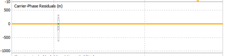
Below I have plotted the fractional part one of the phase-bias estimate differences for the three cases. The discontinuity at 180 seconds is where fix-and-hold and fix-and-bump were enabled. The plot on the right is just a zoomed-in version of the plot on the left.

Here is the solution stats for each run. (1=float, 2=fix,3=hold)

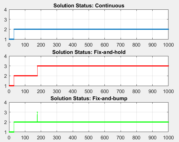
As you can, even a single adjustment (fix-and-bump) gives us an estimate of the phase-bias that is very close to what we get if we make adjustments every epoch (fix-and-hold). This supports the idea that it may be possible to get most of the benefit of fix-and-hold while avoiding some of the downside.

At this point, this is more of a thought exercise, than a proposal to change RTKLIB but I think it may be worth considering. I hope to evaluate this change further when I have more data sets to look at.

I will use this feature though in my next post, though, which is one reason I’ve devoted a fair bit of time to it here. In that post I will extend fix-and-bump to the GLONASS satellites. Instead of using the feedback short-circuit path (as I’ve called it) to improve the phase-bias estimates, I will use it to estimate the inter-channel biases, then enable GLONASS integer ambiguity resolution. Not having the inter-channel bias values is what currently prevents integer ambiguity resolution (gloarmode) for the GLONASS satellites from working. Fix-and-bump should provide better evaluation of the quality of the combined GPS/GLONASS solutions.  That’s enough for now … I’ll leave the rest to the next post.

Note:  Readers familiar with the solution algorithms will notice that I have left out certain details and that some of my statements are not quite precisely correct. For the most part this was done intentionally to keep things focused but I believe the gist of the argument is valid even when all the details are included. Please let me know if you think I have left anything important out.

Evaluating results: Moving base vs fixed base

 

In the last few posts, I have been focusing on the relative position solution between two receivers where both are moving but fixed relative to each other rather than the more typical scenario where one receiver is fixed (the base) and the other is moving (the rover). As described in an earlier post, I do this because it makes it possible to accurately measure the error in the solution when we don’t have an absolute trajectory reference to compare to.

Normally, though, from a functional viewpoint, we are more interested in the second case where one receiver is fixed and the other is moving. In this post I will spend a little time looking at how we can evaluate the results for that scenario.

Since we don’t know what our exact trajectory was when we collected the data, we can not measure our solution error directly like we can in the first case. However, we can look for consistency between multiple solutions calculated for the same rover data, but with varying input configurations and differing base data and satellites. The solution should not vary by more than our error tolerance no matter how much we change the input configurations.  If we believe a solution is accurate to a couple of centimeters then it would be very disturbing to find it moved 50 cm if we used the same rover data but adjusted something in the input configuration, satellites, or base data, particularly if the differences occur for epochs with fixed solutions.  We cannot know which of the two solutions is incorrect but we do know that at least one of them must have large undetected errors in it, which means we really can’t trust either solution. Of course, if the two solutions are equal it does not guarantee that they are correct, they may just both be wrong in the same way. However, the more we can vary the input conditions and still get the same answer, the more confident we will start to have in the solution.

To test the consistency of solution for the previous data set, I processed the data from the two receivers in a different way. Instead of measuring the relative distance between the two receivers, I measured the distance between each receiver and two independent base stations, giving me a total of four solutions, two for each Ublox receiver Since the two base receivers are in different locations the solutions will be different, but if we ask RTKLIB to calculate absolute position rather than relative distance then we can compare the two directly. By changing the out-solformat parameter in the input config file from “enu” to “xyz”, RTKLIB will add the absolute location of the base station to the solution, converting it from relative to absolute. With this change, the two solutions calculated from different base stations should be identical.

For the two base receivers, I used data from two nearby stations in the NOAA CORS network, TMG0 which is about 5 km away from where I collected the data and ZDV1 which is about 13 km away. TMG0 data includes Glonass satellites, ZDV does not so this also helps differentiate the two solutions by giving them different but overlapping satellite sets. To further increase the difference between the two satellite sets, I changed the minimum elevation variables in RTKLIB for the TMG station from 15 degrees to 10 degrees while leaving them at 15 degrees for the ZDV station. This will add the low elevation satellites to the TMG solution.

Now we can compare the two solutions for each Ublox receiver, each calculated with different base stations and different sets of satellites. If everything is working properly they should be identical within our expected error tolerance. Since our baseline distances between base and rover have increased from roughly 30 cm in the previous analysis to 5-13 km in this case we will expect the errors to be somewhat larger than they were before.

The plots below show the results of this experiment. The plots on the left are from the Ebay receiver and the plots on the right are from the CSG receiver. The first row of plots show the ground tracks for both solutions overlayed on top of each other, the second row shows position in x, y, and z directions, again for both solutions overlayed on top of each other. The x and y directions are indistinguishable at this scale but we do see some error in the z direction. The third row of plots shows the difference between the two solutions. We can interpret these differences as a lower bound for our error. As we would expect with the longer baselines, the errors are somewhat larger than before, but at least the x and y errors are generally still quite reasonable, most of them falling between +/- 2 cm for epochs with fixed solutions (green). The z errors are somewhat larger but fortunately we usually care less about this direction. I have made no attempt to reduce the ephemeris errors, either through SBAS or precise orbit files. Presumably, at these longer baselines, doing so would help reduce the errors.

So, how do we interpret these results? I believe this analysis is consistent with the previous analysis. It is not as conclusive since we have no absolute error measurement, but since the solutions are more similar in format to how they would be done in practice, it should give us more overall confidence in our results.

Maybe more important, it also provides a baseline for using similar consistency analysis on other data sets where we often won’t have the luxury of having two receivers tracking the same object.

Let me add a few words to help put these results in context in case you are comparing them with other data sets.  This data was all taken in very open skies with fairly low velocities (<6 m/sec) so it is relatively easy data to get a good solution.  It will be more difficult to get similar results for data taken with obstructions from trees or buildings, or that includes high velocities or accelerations or high vibration.  In particular, there were very few cycle slips in this data.   None of the modifications described here will help if the data has a large number of cycle slips.

Also remember that this data was taken with very low cost hardware (the Ebay receiver cost less than $30 for receiver and antenna combined) so the data will be lower quality relative to data taken under similar conditions with more expensive hardware, especially higher quality antennas.  

That is the goal of my project, though, to get precise, reliable positioning with ultra-low cost hardware under benign environmental conditions. 

 

 

 

 

Improving RTKLIB solution: Phase-bias sum error

While working through the code to add comments as described in the last post, I stumbled across what looks like another bug. This one is more subtle than the previous bug (arlockcnt) and only has a small effect on the results, but still I thought it was worth discussing.

During each epoch, RTKLIB estimates the phase-bias for each satellite using the differences between the raw carrier-phase measurements and the raw pseudorange measurements. In a perfect system, these should always differ by an integer number of cycles because the carrier-phase measurement have an uncertainty in the number of cycles whereas the pseudorange measurements do not. These phase-bias estimates are then used to update the kalman filter.

Before updating the kalman filter however, RTKLIB calculates the common component between all satellites and subtracts this off of each phase-bias states (the kalman filter outputs) My guess is that this code is left over from the GPS-only days where all satellites operated at the same frequency since the estimates are all in units of cycles. As long as the frequencies of each satellite are identical, it is fine to add the cycles from one satellite to another, but this doesn’t work anymore once the satellite cycles are of different frequencies.

My code modification simply converts the biases to meters first using the wavelength for each satellite before summing them and then converting back to cycles for each satellite. The changes all occur in the udbias() routine. The following lines of code:

1) bias[i]=cp-pr/lami;

2) offset+=bias[i]-rtk->x[IB(sat[i],f,&rtk->opt)];

3) if (rtk->x[IB(i,f,&rtk->opt)]!=0.0) rtk->x[IB(i,f,&rtk->opt)]+=offset/j;

become

1) bias[i]=cp*lami-pr;

2) lami=nav->lam[sat[i]-1][f];
    offset+=bias[i]-rtk->x[IB(sat[i],f,&rtk->opt)]*lami;

3)   if (rtk->x[IB(i,f,&rtk->opt)]!=0.0) {
       lami=nav->lam[i-1][f];
      rtk->x[IB(i,f,&rtk->opt)]+=offset/lami/j;
     }

This improves the solution slightly but is most obvious when the receiver does a clock update. Since the receivers use inexpensive crystal clocks, unlike the satellites which use atomic clocks, there is a continuous drift between the two. At some point, when the difference between these two clocks gets too large, the receiver will update its clock to remove the error. Most of the time the error introduced by this bug is too small to easily pick out of the noise, but when there is a large adjustment from the clock correction it becomes quite obvious and shows up as a large spike in the residuals. Adding this code change eliminates the spikes from the residuals.

While exploring this issue, I modified the code that outputs to the state file to also output the phase-biases since I felt they provided a fair bit of insight to what was happening in the solution. What I found however when looking at these phase-bias outputs is that they are dominated by this common term (presumably some sort of clock bias) and it is difficult to see the behavior of the individual phase biases. To avoid this problem I made another modification to the code. Instead of adding the common component to every phase-bias state, I saved it in a separate common bias variable and used this when initializing phase-biases for new satellites. Since all position calculations are done with the difference of the phase-biases and not the phase-biases themselves, this change does not have any effect on the output solution. It does however remove the large common variation from the phase-bias states and makes them easier to analyze.

Here are the residuals before and after the code modification (zoomed way out to see the spike).

The position solution doesn’t change much, the improvement is more obvious in the confidence of the solution which can be seen in the Ratio Factor for AR validation. Here it is before (green) and after (blue) the code modification.

As you can see there is a small but persistent increase in the AR ratio with this change.

Anyone else run across this issue and solved it in a different way? Or believe this is not a bug, and is actually the intended behavior? Or possibly know of other cases where cycles of different wavelengths are not handled properly in RTKLIB?

RTKLIB: Code comments + new Github repository

If you’ve spent any time perusing the RTKLIB source code you will surely be aware that it is very much what I would call “old-school” code. Comments are sparse and variable names tend to be short and not always very descriptive. The upside is that the code is quite compact, significant pieces of it can be seen on a single page which can sometimes be quite nice. The downside is it can be difficult to follow if you have not been poring over it for a long time. To help myself understand the code I have added a fair bit of commenting to most of the code used to calculate the carrier-phase solution, which is really the heart of the RTKLIB kinematic solution.  This is mostly in the rtkpos.c file.

The changes are too extensive to spell out here so I have forked the RTKLIB code in Github and posted my commented code there. If you are interested, you can download it from the demo1 branch at https://github.com/rtklibexplorer/RTKLIB.  

All the previous code changes are also there as well as a couple I have not yet posted about.  The receiver data I have been using for these posts is also there in the rtklib/data/demo1 folder.  The solution file updates for VS2010 c++ are in the rtklib/app/rnx2rtkp/msc folder and the modified executable is in the rtklib/bin folder.

Improving RTKLIB solution: (AR lock count and elevation mask)

In the previous post, after a couple changes to the input parameters, we ended up with the following solution for the difference between two stationary, then moving Ublox receivers:

During the time when the receivers were stationary (17:25 to 17:45), we were able to hold a fixed solution (green in plot) continuously after the initial convergence, but started to revert to float solution (yellow in plot) fairly frequently once the receivers started moving.

Let’s look at the data a little closer to see if we can discern why we are reverting back to the float solution. If we switch to the “Nsat” view in RTKPLOT plotted below, we can see a couple of useful plots.

The top plot shows the number of satellites used for the solution and the bottom plot show the AR ratio factor. The AR ratio factor is the residuals ratio between the best solution and the second best solution while attempting to resolve the integer cycle ambiguities in the carrier-phase data. In general, the larger this number, the higher confidence we have in the fixed solution. If the AR ratio exceeds a set threshold, then the fixed solution is used, otherwise the float solution is used. I have left this threshold at its default value of 3.0.

Notice in the plot that each time we revert to the fixed solution, it happens when the number of valid satellites increases. At first this seems counter-intuitive, you would think that more information would improve the solution, not degrade it. What is happening though, is that the solution is not using the satellite data directly, but rather, the kalman filter estimate of the data. This estimate improves as the number of samples increases. This is also why the solution takes some time to converge at the beginning of the data. By using the data from the new satellite before the kalman filter has had time to converge, we are adding large errors to the solution, forcing us back to the float solution.

Fortunately, RTKLIB has a parameter in the input configuration file to address this issue. “Pos2-arlockcnt” sets the minimum lock count which has to be exceeded before using a satellite for integer ambiguity resolution. This value defaults to zero, but let’s change it to 20 and see what happens. While we are it, we will also change the related parameter “pos2-arelmask” which excludes satellites with elevations lower than this number from being used. We will change this from it’s default of 0 to 15 degrees.

Unfortunately, re-running the solution with these changes makes almost no difference as seen below. The jumps back to float solutions still occur immediately after a new satellite is included, and the additional satellites are being included at the same epochs. Something is clearly wrong.

 

Digging into the code a bit reveals the problem. First, the arlockcnt input parameter is copied to a variable called “rtk->opt.minlock” Then the relevant lines of code from rtkpos.c are:

rtk->ssat[sat[i]-1].lock[f]=-rtk->opt.minlock;

if (rtk->ssat[i-k].lock[f]>0&&!(rtk->ssat[i-k].slip[f]&2)&&
     rtk->ssat[i-k].azel[1]>=rtk->opt.elmaskar) {
     rtk->ssat[i-k].fix[f]=2; /* fix */
     break;
}
else rtk->ssat[i-k].fix[f]=1;

So far, everything looks OK, but when we look at the definition for the structure member “lock” in rtklib.h we find:

unsigned int lock [NFREQ]; /* lock counter of phase */

This won’t work. We are assigning a negative number (-rtk->opt.minlock) to an unsigned variable, then checking if the unsigned variable is greater than zero, which by definition, will always be true. Hence, satellites are always used immediately, regardless of lock count.

We fix this bug by changing the definition of lock from unsigned to signed:

int lock [NFREQ]; /* lock counter of phase */

Rerunning after rebuilding the code, gives us the following solution:

Much better! All but a couple of the jumps back to float solutions have been eliminated.

Looking at the plot of the AR ratio for this solution, we can see that the kalman filter requires more than 20 seconds (the value we chose for arlockcnt) to re-converge. Two minutes looks like a more reasonable value from the plot, so let’s try rerunning the solution with arlockcnt=120.

Even better.  That eliminates the last couple of jumps back to the float solution and also significantly reduces the number of jumps in the AR ratio plot as shown below. The green line in the bottom plot is arlockcnt=20 and the blue line is arlockcnt=120.

It’s possible we will need to revisit this number after looking at more data, but for now we will use 120 secs.

As always, please leave a comment if you have any comments, discussion points, or questions.

Update 4/11/16:  

• In the above discussion, my data is one epoch/sec and I equate epochs with seconds.  Arlockcnt is specified in epochs, not seconds, so if your data is at a different sample rate you will need to adjust accordingly.
• The suggestion above to set arlock to 120 secs is probably too conservative for more challenging environments.  If there are few satellites and/or many cycle slips for example it is probably better to start using a just-locked satellite before it is fully converged.  I have started using 30 secs rather than 120 secs for my solutions.
• You can pull this code fix from my github repository either by itself from the arlockcnt branch or as part of a larger set in the demo1 branch

Improving RTKLIB solution: (Receiver Dynamics and Error Ratio)

In the previous posts, I demonstrated reasonably clean looking solutions using the default RTKLIB configuration options for rover data from a roving M8N receiver and base data from a stationary COREX base station.

I also showed a second solution for the slightly more challenging problem where roving M8N receivers are used for both the base and rover inputs. I mentioned that run was not done with the default settings but did not go into the details. Let us now go back and try that run using the default settings and see what happens. Remember what we hope to see is a circle with radius equal to the separation between the two receivers, ideally plotted in green, indicating RTKLIB was able to resolve the integer ambiguities and provide a fixed solution.

For reference, here is the solution we previously calculated with RNX2RTKP using non-default settings and code. The plot on the left is from the ground track option in the RTKPLOT menu which plots the x axis vs the y axis and the second plot is the position option which plots all 3 directions separately vs time.

Below is what we get running with the default settings with the two basic modifications I mentioned earlier. The red indicates the kinematic solution is unable to converge and the plotted result is done in single mode, which is not differential, and therefore is indicating absolute position, and not distance between the two receivers.

Clearly, the default settings are not adequate when both receivers are lower quality and both are moving. Let’s see if we can improve this.

First, let’s make a few small changes that won’t improve the solution but will make the input assumptions better match our problem.

Edit the input configuration file for rnx2rtkp to make the following changes. These are in addition to the two changes we made earlier (pos1-posmode and ant2-postype)

1. pos1-frequency: L1+L2 → L1, both receivers are L1 only, so no need to look for L2 data
2. pos1-navsys: 1 → 5, we have GLONASS data, so let’s use it
3. pos2-gloarmode: on->off, not ready for this yet, in current state, it prevents fixed solution
4. pos2-bdsarmode: on->off, no Bediou data so disable
5. out-solformat: llh → enu, save solution to output file with equal units in x and y axis
6. out-outstat: off → residual, save residuals for later analysis

Rerunning RNX2RTKP gives us a solution very similar to the previous one with little improvement, even with the additional data from the GLONASS satellites.  I won’t bother to plot it here.

Next, let’s turn on receiver dynamics with the “pos1-dynamics” input option. This adds nine states to the kalman filter, 3 for receiver position, 3 for velocity, and 3 for acceleration. This enables the solution to take into account the previous position of the receiver when calculating the new solution and allows us to better define likely changes in position, velocity, and acceleration. For now, we will use the default filter settings. With this change, the solution looks like this:

Not quite there yet, but much better. We can now see the expected circle but there are fairly large errors when the solution is not fixed. We do sometimes resolve the integer ambiguities but only 26.6% of the time.

Next, we’ll take a very brief look at the input parameters defining the error characteristics of the input data. For the kalman filter to effectively combine the data from multiple inputs, it requires information about the error distribution of each input.  RTKLIB calculates the variances of each code and carrier phase input based on a set of input parameters and a simple model based on satellite elevation, the assumption being that lower elevation satellites are noisier. For now, we will look at only the first input parameter. This is “stats-eratio1” and it sets the ratio of standard deviations of the pseudorange errors to the standard deviations of the carrier-phase errors. I believe it is not unreasonable to expect, with the lower quality receiver and antenna we are using, that the pseudorange errors will degrade more quickly than the carrier-phase errors. If this is true, then it would make sense to increase this ratio from the default of 100. Setting this to 300 give the following solution.

This looks a lot better. We converge much more quickly to a fixed solution and when it loses lock it also re-converges more quickly.

We still need to make a few more changes to get to the quality of the solution at the top of this post, but most of those changes require making some code changes so I will leave them to another post.

The physical justification for using 300 for the error ratio is a bit weak at this point but we’ll just go with it for now and I hope to come back and do a more complete analysis of the way RTKLIB generates the variances and covariances for input to the kalman filter later.

Anyone else come up with a good way to optimize the  RTKLIB input parameters for the kalman filter convariances?  If so, please leave a comment, I’m interested in how other people handle this problem.

Update 6/12/16:  Since writing this post, I have found that increasing eratio1 can have a tendency to increase the number of false fixes if “pos2-rejionno” is not also increased at the same time.  I now recommend that if you increase eratio1 that you also increase rejionno from 30 to 1000.  This should eliminate false rejection of outliers.  For more details see this post.

 

Building RTKLIB 2.4.3 code with Visual C++ 2010

One of my goals in this project is to make some changes to the RTKLIB solution algorithms and evaluate them specifically for my set of inputs. RTKLIB is intended to work in many different environments. I would like to customize it to be optimal for calculating differential solutions for two single frequency receivers assuming low velocities and open skies. Some of the changes I would like to make are based on what other people have already tried but for which code is not available. Other changes are based on looking at cases in my data where RTKLIB did not provide a good solution, understanding why, and changing the algorithm appropriately.

To make these changes, I need to be able to modify the RTKLIB code and rebuild it. Since I am doing this initial evaluation work on a Windows PC I will need to build the code in that environment. The GUI versions of the RTKLIB programs require the Embarcadero C++ compiler which I do not have and which is fairly expensive to purchase. The CUI versions can be built with Visual C++, which is available for free, so I have chosen to go that path. As mentioned before, I also find the CUI interface with a matlab wrapper better for tracking configuration information for multiple runs.

The project files for Visual C++ are in the rtklib\app\”app name”\msc folders. They are configured for Visual C++ 2008. Since I already have Visual C++ 2010 loaded on my machine I had to make a few changes to make the project files work. Some of the changes would also be required with VS 2008 since it does not look like the project files have been kept up to date with recent RTKLIB changes.

1. Convert solution files to VS 2010: Click on msc.sln file in rtklib\app\rnx2rtkp\msc folder. This will bring up the visual studio conversion wizard which will convert the VC 2008 project files to VC 2010.
2. Add new src files to project: Add tides.c and ppp_corr.c to the list of source files in the “Solution Explorer” window by right-clicking on the source folder and selecting “Add”. This prevents build errors from unfound symbols.
3. Modify Include Directories: Select “Properties” from “Project” tab. Select “General” under “C/C++” under “Configuration Properties” in the menu on the left hand side. Replace the existing entry with “..\..\..\src” to make it independent of code path. This enables the compiler to find the rtklib.h file.
4. Modify Target Name: Select “General” under “Configuration Properties” in the the menu on the left hand side and change “Target Name” to “rnx2rtkp” to avoid linking errors.
5. Add winmm library: Select “Input” under “Linker” under “Configuration Properties” in the menu on the left hand side, and add “winmm.lib” to “Additional Dependencies”. This avoids linker errors for an unresolved TimeGetTime symbol.
6. Fix LPCWSTR conversion warning: Select “General” under “Configuration Properties” in the the menu on the left hand side and change “Character Set” from “Use Unicode” to “Not Set”

To run these apps from the data folders you will need to add the paths for the executables to your Windows path variable. The executables are in app/”app name”/Release/”app name”.exe or app/”app name”/Debug/”app name”.exe depending on whether you built in Debug or Release mode. I always build in Debug mode and point my path variable to that folder just to make it easier to switch between debugging with VS and running stand-alone, but either will work.

Evaluating the quality of moving position solutions

Stationary position solutions are easy to evaluate, an ideal solution is a single point, any deviation from this point must be error. It is possible that the point itself is in error in an absolute sense but since I am only interested in the distance between receivers I am not concerned with absolute error.

Evaluating a solution for a moving receiver is more difficult since it is not easy to know what is the correct solution to compare to. If I had an expensive high precision receiver/antenna I could mount it on the same platform as the test receiver and use that as a reference, but I don’t have that, so I need to come up with another solution.

Mounting two low cost receivers on the moving platform gives us a couple of options for evaluation. First of all, since I have data from two nearby base stations, I can calculate two solutions, each using one of the low cost moving receivers as rover, and one of the COREX base stations for base data. Since the two low cost receivers remain a fixed distance apart, the difference between the two solutions should be constant in magnitude. The direction of the difference however is varying as the orientation changes. This means the difference between the two solutions should be a circle with radius equal to the distance. Since each solution is based on different base stations, and different receivers they should be fairly independent. The fact that one of the base stations is reporting GPS only, and the other is reporting GPS and GLONASS should also increase the independence of the solutions, since they are also using different sets of satellites,at least if we include GLONASS satellites in the solution. This not the case at the moment since the default config has GLONASS turned off, but we will turn it on soon.

RTKPLOT has a nice feature which allows us to plot the difference between two solutions. Click on the “1-2” button on the menu bar to see this, after opening both solutions from the file menu.

Below are the two solutions plotted on top of each other. Since the scale is 20 meters per division, it is impossible to see any difference between them.

Here is a plot of the difference between the two solutions while the car was stationary and driving in low velocity circles. Now the scale is 10 cm per division. We can see the expected circle, and the error from that circle is generally less than 5 cm once the solution converges to a fixed solution. I’ve jumped ahead a bit, since the solution in the plots includes some input parameter changes as well as some code changes, so the default solution we just calculated won’t be as clean, but we’ll get to those changes soon. The good news is that it looks like we are getting errors of only a few centimeters after the solution has converged, even when both receivers are moving.

There is also another, simpler way to evaluate the quality of the solutions if, as in my case, we are interested only in relative error and not absolute error. Instead of generating absolute solutions using the COREX base stations, we can calculate a differential solution directly, using one of the low-cost receivers as the base and the other as the rover. The result will then be the position difference between the two receivers. Since the distance between the two receivers is fixed but the orientation between them is varying as the platform they are on is moving, the solution should be a circle, again with radius equal to the distance between the two receivers. In this case, unlike the previous one, we do not get any absolute position information, only the distance between the two receivers. Note that even though the base is moving in this case, we do not use the “Moving-Base” solution option from the positioning mode choices, but stick with “Kinematic”. The solution algorithm does not need exact position of the base, only approximate location. We use the approximate starting location of the base receiver which is in the header of the RINEX observation file and ignore the fact that the base is moving. As long as we are concerned only with relative position between the two receivers and the base does not move a large distance from its starting point, this is a valid assumption to make.

Here is a plot of the result from using both base and rover on the moving platform. Note that it is very similar to the previous plot, generated from the difference between two absolute solutions, and again the error is only a few centimeters once the solution has converged.  As in the last plot, it does include some changes from the default input parameters and code that we will get to later.

This is the form of solution I will use for evaluating the effectiveness of various input parameters and algorithm changes.

Kinematic solution with RNX2RTKP

 

In the last post we used the RTKPOST GUI to generate a kinematic position solution using “ebay.obs” for the rover data and “zdv13480.15o” for the base station data. To do the equivalent run from RNX2RTKP we use the following command line, run from the folder containing the data files.

rnx2rtkp -k test1.conf -o out.pos ebay.obs zdv13480.15o ebay.nav

The -k option is to specify the configuration file, the -o option is the output file. In this case we use the configuration file we saved from RTKPOST in the previous post.

To plot the calculated solution use the following command line:

rtkplot out.pos

This calls up the same plot GUI we previously accessed by clicking on the “Plot” button in the RTKPOST GUI.

The plots should be identical between this solution and the previous solution generated with RTKPOST.

To keep track of changes between various runs with the same data, I use a matlab wrapper to create a sub-folder, copy the config file, trace file, stats file, and result file to that sub-folder, input a short description of the run, and also save that to the sub-folder.

Kinematic solution with RTKPOST

Kinematic solution with RTKPOST

RTKPOST is the GUI tool in RTKLIB to calculate position solutions. Most of the time I find the CUI version (RNX2RTKP) better fits my needs, but just to check everything is working, it is probably easier to use RTKPOST the first time.

For a demonstration of using RTKPOST to find a kinematic position solution, I will use the ZDV1 (COREX station data) for base station data and the “EBAY” (Ublox M8N receiver data) for rover data. Zipped versions of this data is available here. (Update 1/24/20:  This data is no longer available, but similar data can be downloaded from  here.)  Since the exact location of ZDV1 is known and is in the observation file header, the kinematic solution will give us an absolute position by solving for the relative distance between the rover and the base, and then adding that to the base location. I set up the GUI inputs as shown below to point the program to the correct observation and navigation files. If you use my data, be sure to change the paths to match where you saved the data to.

For this first run, to keep things as simple as possible, we will make just two changes from the default setup. Use the “Options” button to get to the options menu. Under the “Setting 1” tab, change “Positioning mode” from “Single” to “Kinematic”. This will give us a differential solution using carrier phase info instead of an absolute solution using only pseudorange. Next, under the “Positions” tab, change the first field under “Base Station” from “Lat/Lon/Height” to RINEX Header Position. This will tell RTKPOST to get the base station location from the header of the observation file.

While you are in the options menu, click the “Save” button, and save the options setup to a location you will remember later. We will use this file as the configuration input file for the CUI version. Then click OK to exit the Options menu.

Click the “Execute” button to calculate position and then “Plot” to see the solution. Select “Gnd Trk” and zoom in and it should look like this. The two rectangles are parking lots. The yellow represents a float solution, the green a fixed solution. The fact that we were able to get a fixed solution at least part of the time is a sign things are working reasonably well.

Zooming into the initial time period when the car was stationary we see the plot below. Since the receiver is not moving during this time, any movement in the solution represents error. During the initial convergence of the kalman filter we see quite a lot of error, but once it does converge, we do get a fixed solution for 5 of the 20 minutes which appears as green in the plot below. During this time you can see the error is roughly +/- 1cm in the xy direction which again is a good sign things are working.

Note about restoring RTKPOST default options:  There is no button in RTKPOST to reset the options to defaults and it remembers the options from the previous session when restarted, so there is no obvious way to put it back to defaults.  The best way I have found to do this is to delete the “rtkpost.ini” file saved in the rtklib\bin folder before starting RTKPOST.